%%{init: {'theme':'base', 'themeVariables': {'primaryColor':'#2C3E50','primaryTextColor':'#fff','primaryBorderColor':'#16A085','lineColor':'#16A085','secondaryColor':'#E67E22','tertiaryColor':'#ECF0F1','fontSize':'13px'}}}%%
flowchart TD
Power[Battery Power Budget<br/>2000 mAh]
L1[Level 1: Reduce Wi-Fi Transmissions<br/>80% of power budget<br/>16 mAh/day savings]
L2[Level 2: Connection Optimization<br/>15% of power budget<br/>3 mAh/day savings]
L3[Level 3: Protocol Efficiency<br/>3% of power budget<br/>0.6 mAh/day savings]
L4[Level 4: Sensor Sampling Reduction<br/>2% of power budget<br/>Last resort - reduces data quality]
S1[Buffer readings<br/>Transmit every 2 hours]
S2[Keep-alive optimization<br/>MQTT persistent sessions]
S3[CoAP vs HTTP<br/>Lightweight protocols]
S4[Reduce sample rate<br/>15 min to 1 hour]
Power --> L1
Power --> L2
Power --> L3
Power --> L4
L1 --> S1
L2 --> S2
L3 --> S3
L4 --> S4
style Power fill:#2C3E50,stroke:#16A085,color:#fff
style L1 fill:#c0392b,stroke:#2C3E50,color:#fff
style L2 fill:#E67E22,stroke:#2C3E50,color:#fff
style L3 fill:#f39c12,stroke:#2C3E50,color:#fff
style L4 fill:#16A085,stroke:#2C3E50,color:#fff
style S1 fill:#16A085,stroke:#2C3E50,color:#fff
style S2 fill:#16A085,stroke:#2C3E50,color:#fff
style S3 fill:#16A085,stroke:#2C3E50,color:#fff
style S4 fill:#16A085,stroke:#2C3E50,color:#fff
552 Sensor Networks and Power Management
Multi-Sensor Aggregation and Battery Optimization
sensing
power-management
low-power
networks
Keywords
power management, deep sleep, battery life, sensor networks, duty cycling, ESP32 sleep
552.1 Learning Objectives
By the end of this chapter, you will be able to:
- Design multi-sensor data aggregation systems with structured JSON payloads
- Calculate power budgets for battery-powered sensor nodes
- Implement deep sleep modes for microamp-level current consumption
- Optimize transmission strategies to extend battery life by 3-5x
- Apply sensor fusion concepts to combine complementary sensor data
552.2 Introduction
Battery-powered IoT sensor nodes face a fundamental challenge: they must collect and transmit data reliably while consuming minimal power. A well-designed power management strategy can extend battery life from weeks to years. This chapter covers the techniques that make long-term remote sensing practical.
TipMinimum Viable Understanding: Sensor Fusion
Core Concept: Sensor fusion combines data from multiple sensors (e.g., accelerometer + gyroscope + magnetometer) using algorithms like complementary filters or Kalman filters to produce more accurate and reliable measurements than any single sensor alone.
Why It Matters: Individual sensors have inherent limitations - accelerometers drift over time, gyroscopes accumulate integration errors, and magnetometers are affected by nearby metals - but fusing their outputs compensates for each sensor’s weaknesses while amplifying their strengths.
Key Takeaway: Start with a simple complementary filter (weighted average of fast and slow sensors) for orientation sensing - it requires only 5 lines of code and achieves 80% of Kalman filter accuracy without the computational complexity or tuning challenges.
552.3 Multi-Sensor Data Aggregation
Combining multiple sensors into a single IoT node requires structured data handling. JSON payloads provide a flexible, human-readable format for transmitting aggregated sensor data.
#include <DHT.h>
#include <Wire.h>
#include <BH1750.h>
#include <Adafruit_BMP280.h>

DHT dht(4, DHT22);
BH1750 lightMeter;
Adafruit_BMP280 bmp;

struct SensorData {
  float temperature;
  float humidity;
  float pressure;
  float altitude;
  float light;
  unsigned long timestamp;
};

void setup() {
  Serial.begin(115200);
  Wire.begin();

  dht.begin();
  lightMeter.begin();
  bmp.begin(0x76);
}

SensorData readAllSensors() {
  SensorData data;

  data.temperature = dht.readTemperature();
  data.humidity = dht.readHumidity();
  data.pressure = bmp.readPressure() / 100.0;
  data.altitude = bmp.readAltitude(1013.25);
  data.light = lightMeter.readLightLevel();
  data.timestamp = millis();

  return data;
}

void loop() {
  SensorData data = readAllSensors();

  // Create JSON payload
  String json = createJSON(data);
  Serial.println(json);

  // Publish to MQTT or send via HTTP
  publishData(json);

  delay(10000);
}

String createJSON(SensorData data) {
  String json = "{";
  json += "\"temperature\":" + String(data.temperature) + ",";
  json += "\"humidity\":" + String(data.humidity) + ",";
  json += "\"pressure\":" + String(data.pressure) + ",";
  json += "\"altitude\":" + String(data.altitude) + ",";
  json += "\"light\":" + String(data.light) + ",";
  json += "\"timestamp\":" + String(data.timestamp);
  json += "}";

  return json;
}
552.4 Low-Power Sensor Reading
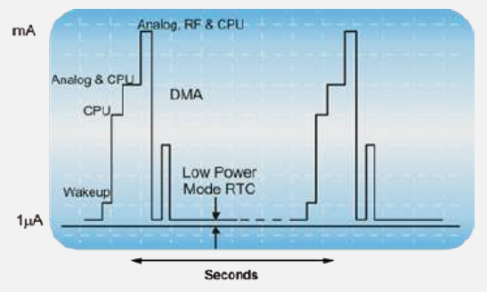
Deep sleep modes reduce current consumption from milliamps to microamps, dramatically extending battery life.
#include <esp_sleep.h>

#define SLEEP_DURATION 60  // seconds

void setup() {
  Serial.begin(115200);

  // Read sensors
  float temperature = readTemperature();

  // Send data
  sendDataToCloud(temperature);

  // Enter deep sleep
  Serial.println("Entering deep sleep...");
  esp_sleep_enable_timer_wakeup(SLEEP_DURATION * 1000000);  // microseconds
  esp_deep_sleep_start();
}

void loop() {
  // Not used - device resets after deep sleep
}

552.5 Power Budget Calculation
Understanding power budgets is essential for designing battery-powered sensor nodes. Let us calculate the battery life for a typical environmental monitoring node.
552.5.1 Example: Weather Station Power Analysis
System Configuration:
- ESP32 with BME280 sensor
- LoRa transmission every 15 minutes
- 2000 mAh battery
Current Consumption:
| State | Current | Duration per Cycle |
|---|---|---|
| Active (sensor read + LoRa TX) | 150 mA | 5 seconds |
| Deep Sleep | 10 uA | 895 seconds |
Calculation:
Active Period Energy:
  150mA × (5/3600)h = 0.208 mAh per cycle

Sleep Period Energy:
  0.01mA × (895/3600)h = 0.0025 mAh per cycle

Total per 15-minute cycle: 0.21 mAh

Cycles per day: 96

Daily consumption: 96 × 0.21 = 20.2 mAh/day

Battery life: 2000mAh / 20.2 mAh/day = 99 days
552.5.2 Optimization Strategy: Transmission Buffering
The biggest power consumer is Wi-Fi/LoRa transmission. Buffering multiple readings before transmitting dramatically reduces power consumption.
Original approach: 96 transmissions/day
Buffered approach (transmit every 2 hours): 12 transmissions/day
#define READINGS_PER_TX 8
float tempBuffer[READINGS_PER_TX];
int bufferIndex = 0;

void loop() {
    // Read sensor (fast, low power)
    tempBuffer[bufferIndex++] = bme.readTemperature();

    if (bufferIndex >= READINGS_PER_TX) {
        // Transmit all buffered readings
        connectWiFi();
        sendAllReadings(tempBuffer, READINGS_PER_TX);
        disconnectWiFi();
        bufferIndex = 0;
    }

    esp_deep_sleep(15 * 60 * 1000000);  // 15 minutes
}
Power savings:
- Wi-Fi transmissions: 96 to 12 per day (87.5% reduction)
- Wi-Fi energy: 16 to 2 mAh/day
- New battery life: 322 days (3.3x improvement)
552.5.3 Power Optimization Hierarchy
552.6 Sensor Fusion Tradeoffs
WarningTradeoff: Complementary Filter vs Kalman Filter for Sensor Fusion
Option A: Complementary Filter - Simple weighted combination using high-pass filter on one sensor and low-pass filter on another (e.g., gyroscope + accelerometer for orientation)
Option B: Kalman Filter - Statistically optimal recursive estimator that models system dynamics, measurement noise, and process noise for state estimation
Decision Factors:
| Factor | Complementary Filter | Kalman Filter |
|---|---|---|
| Computational load | Very low (few multiplies) | High (matrix operations) |
| Memory footprint | ~20 bytes | 200-2000 bytes |
| Tuning complexity | 1-2 parameters | 5-20+ parameters |
| Accuracy | Good (80-90% of optimal) | Optimal (by definition) |
| Sensor modeling | Assumes fixed noise | Adapts to varying conditions |
| Latency | Minimal | Slight (prediction step) |
| Implementation time | Hours | Days to weeks |
Choose Complementary Filter when: Constrained MCU (8-bit AVR, small ARM Cortex-M0); battery life critical; quick prototyping; simple sensor fusion (2-3 sensors); accuracy requirements modest.
Choose Kalman Filter when: Accuracy is paramount; sensors have varying reliability over time; need state prediction between measurements; tracking moving targets; fusion of many sensors (5+); adequate computational resources available.
Practical guideline: Start with complementary filter for proof-of-concept. If accuracy is insufficient, upgrade to Kalman.
WarningTradeoff: Smart Sensors vs Raw Sensors with External Processing
Option A: Smart Sensors - Sensors with on-chip intelligence including calibration, digital output, threshold detection, and sometimes embedded ML (e.g., BNO055 with on-chip sensor fusion, MAX30102 with SpO2 algorithm)
Option B: Raw Sensors + External MCU - Basic analog/digital sensors where all processing, calibration, and fusion happens in your microcontroller (e.g., MPU6050 raw mode + custom fusion code)
Decision Factors:
| Factor | Smart Sensors | Raw Sensors + MCU |
|---|---|---|
| Host MCU load | Minimal (data ready) | High (continuous processing) |
| Algorithm control | Vendor black-box | Full transparency |
| Calibration | Factory-set | Custom per-unit possible |
| Latency | Fixed (sensor-determined) | Configurable |
| Cost per unit | Higher ($5-$30) | Lower ($1-$10) |
| Power (total system) | Often lower | Often higher |
| Debugging visibility | Limited | Full access |
| Algorithm updates | Firmware upgrade (rare) | OTA software update |
Choose Smart Sensors when: Rapid development required; limited MCU resources; vendor algorithm is proven for your use case; consistent behavior across units needed.
Choose Raw Sensors when: Custom algorithms required (proprietary IP, research); maximum flexibility for parameter tuning; need visibility into intermediate values; cost-optimized high-volume production.
552.7 Common Power Pitfalls
CautionPitfall: Entering Deep Sleep Without Configuring Wake Sources First
The Mistake: Calling deep sleep functions (ESP32’s esp_deep_sleep_start(), STM32’s HAL_PWR_EnterSTOPMode(), nRF52’s sd_power_system_off()) without configuring a valid wake source, causing the device to sleep forever and require manual reset or power cycle to recover.
Why It Happens: Deep sleep disables most peripherals and CPU activity to achieve microamp-level current consumption. Unlike light sleep, there is no automatic wake on timer expiration unless explicitly configured. Developers test with short delays during development, then remove the delay for “production” without adding proper wake sources, bricking the device.
The Fix: Always configure at least one wake source BEFORE entering deep sleep:
// WRONG: Entering deep sleep with no wake source (ESP32)
esp_deep_sleep_start();  // Device sleeps forever! Requires power cycle.

// CORRECT: Configure timer wake source (10 seconds)
esp_sleep_enable_timer_wakeup(10 * 1000000);  // 10 seconds in microseconds
esp_deep_sleep_start();

// CORRECT: Configure external interrupt wake (GPIO 33, active LOW)
esp_sleep_enable_ext0_wakeup(GPIO_NUM_33, 0);  // Wake when GPIO33 goes LOW
esp_deep_sleep_start();

// CORRECT: Multiple wake sources (timer OR button)
esp_sleep_enable_timer_wakeup(60 * 1000000);  // 60-second timeout
esp_sleep_enable_ext0_wakeup(GPIO_NUM_0, 0);  // Boot button wake
esp_deep_sleep_start();
Recovery Strategy: During development, always include a “fail-safe” wake source like a 5-minute timer even if primary wake is external interrupt.
CautionPitfall: Reading I2C/SPI Sensor Registers Before Conversion Complete
The Mistake: Reading sensor data registers immediately after triggering a measurement, before the sensor’s internal ADC has completed conversion, resulting in stale data from the previous measurement or invalid values.
Why It Happens: Sensors like the BMP280 (temperature/pressure), ADS1115 (precision ADC), and HX711 (load cell) have multi-millisecond conversion times. The datasheet specifies conversion time, but example code often uses fixed delays or omits waiting entirely. At 400kHz I2C, you can read registers in ~50us, but BMP280 needs 44ms in ultra-high-resolution mode.
The Fix: Check the sensor’s data-ready signal or wait for the specified conversion time:
// WRONG: Reading BMP280 immediately after trigger (44ms conversion!)
bmp.triggerMeasurement();
float temp = bmp.readTemperature();  // Returns PREVIOUS measurement!

// CORRECT: Wait for conversion time (check datasheet)
bmp.triggerMeasurement();
delay(44);  // Ultra-high resolution mode: 44ms
float temp = bmp.readTemperature();

// BETTER: Poll status register for data-ready flag
bmp.triggerMeasurement();
while ((bmp.readStatus() & 0x08) == 0) {
    delayMicroseconds(100);  // Poll every 100us
}
float temp = bmp.readTemperature();
Conversion Times to Know: BMP280 standard: 8ms, ultra-high: 44ms. ADS1115 at 8 SPS: 125ms, at 860 SPS: 1.2ms. HX711 at 10 Hz: 100ms.
552.8 Knowledge Check
Knowledge Check: Power Management Test Your Understanding
Question 1: A battery-powered environmental monitoring node uses an ESP32 with BME280 sensor, transmitting readings every 15 minutes via Wi-Fi. Current consumption is: active mode 150mA (5 seconds), deep sleep 10uA. Using a 2000mAh battery, approximately how long will the node operate?
Click to see answer
Answer: Approximately 75-100 days
Calculation: - Active Period Energy: 150mA x (5/3600)h = 0.208 mAh per cycle - Sleep Period Energy: 0.01mA x (895/3600)h = 0.0025 mAh per cycle - Total per 15-minute cycle: 0.21 mAh - Cycles per day: 96 - Daily consumption: 96 x 0.21 = 20.2 mAh/day - Battery life: 2000mAh / 20.2 mAh/day = 99 daysQuestion 2: What is the most effective way to extend battery life by 3x or more for the node described above?
Click to see answer
Answer: Reduce Wi-Fi transmissions by buffering multiple readings
Wi-Fi transmission dominates the power budget (80%+ of energy). By buffering 8 readings and transmitting every 2 hours instead of every 15 minutes: - Wi-Fi transmissions drop from 96 to 12 per day (87.5% reduction) - Daily energy drops from 20.2 to ~6 mAh - Battery life extends from 99 days to 322+ days (3.3x improvement)
Other options (ESP8266, larger battery, reduced sampling) provide smaller improvements.Question 3: Why must you configure a wake source BEFORE calling esp_deep_sleep_start()?
Click to see answer
Answer: Without a configured wake source, the device sleeps forever and cannot recover without a manual power cycle.
Deep sleep disables the CPU and most peripherals. There is no automatic timeout - the device will remain in sleep mode indefinitely (consuming ~10uA) until a wake event occurs. If no wake source is configured, no wake event can ever occur, and the device is effectively bricked until physically reset.
Always configure at least one wake source (timer, GPIO interrupt, touchpad, or ULP coprocessor) before entering deep sleep.552.9 Summary
This chapter covered power management strategies for sensor networks:
- Multi-Sensor Aggregation: Structured data collection with JSON payloads
- Deep Sleep Modes: Reduce consumption from milliamps to microamps
- Power Budget Calculations: Estimate battery life for design decisions
- Transmission Buffering: Reduce Wi-Fi/LoRa usage by 80%+ for 3x battery life
- Sensor Fusion Tradeoffs: Complementary vs Kalman filters, smart vs raw sensors
- Wake Source Configuration: Critical for deep sleep recovery
552.10 What’s Next
The next chapter covers Sensor Applications, including smart home environmental monitoring, automated blinds control, and temperature-controlled relay systems with practical implementation examples.
NoteRelated Chapters
- Sensor Data Processing - Filtering and calibration
- Sensor Communication Protocols - I2C, SPI interfaces
- Edge Computing - Edge processing patterns