189  Sensor Communication Protocols

189.1 Learning Objectives

By the end of this chapter, you will be able to:

• Compare Serial Protocols: Understand synchronous vs asynchronous serial communication
• Use I2C: Implement two-wire multi-device bus communication for sensor networks
• Use SPI: Configure high-speed synchronous interfaces for fast peripherals
• Use UART: Set up simple point-to-point serial debugging and communication
• Select Protocols: Choose the right protocol based on speed, pins, and device count

189.2 Introduction

Deep dive into sensor-to-microcontroller protocols including I2C, SPI, UART, and system communication methods.

189.3 Sensor Communication Protocols

⏱️ ~20 min | ⭐⭐ Intermediate | 📋 P04.C11.U03

Figure 189.1: Sensor communication protocols overview - serial, I2C, SPI, and wireless interfaces connecting sensors to microcontrollers

Figure 189.2: Synchronous vs Asynchronous serial communication - key differences in clock signal presence and timing coordination

Now that we’ve learned about microcontrollers’ structure and selection criteria, we will consider the appropriate communication protocols for micros to communicate with sensors and other peripherals.

%%{init: {'theme': 'base', 'themeVariables': { 'primaryColor': '#2C3E50', 'primaryTextColor': '#fff', 'primaryBorderColor': '#16A085', 'lineColor': '#16A085', 'secondaryColor': '#E67E22', 'tertiaryColor': '#7F8C8D', 'fontSize': '12px'}}}%%
graph LR
    subgraph Sensor["Sensor Layer"]
        S1["Temp Sensor<br/>(I2C)"]
        S2["Accel Sensor<br/>(SPI)"]
        S3["GPS Module<br/>(UART)"]
    end

    subgraph Gateway["Gateway/MCU"]
        direction TB
        Read["Read Raw<br/>Binary Data"]
        Convert["Convert Units<br/>& Format"]
        Encode["Encode as<br/>JSON/CBOR"]
        Publish["Publish via<br/>MQTT/CoAP"]
    end

    subgraph Transport["Transport"]
        Wi-Fi["Wi-Fi/Ethernet"]
        LoRa["LoRaWAN"]
    end

    subgraph Cloud["Cloud"]
        Broker["Message<br/>Broker"]
        DB["Database"]
    end

    S1 --> Read
    S2 --> Read
    S3 --> Read
    Read --> Convert --> Encode --> Publish
    Publish --> Wi-Fi --> Broker
    Publish --> LoRa --> Broker
    Broker --> DB

    style Sensor fill:#16A085,stroke:#2C3E50,color:#fff
    style Gateway fill:#E67E22,stroke:#2C3E50,color:#fff
    style Transport fill:#7F8C8D,stroke:#16A085,color:#fff
    style Cloud fill:#2C3E50,stroke:#16A085,color:#fff

Figure 189.3: Protocol Translation Flow: Sensors communicate via low-level protocols (I2C, SPI, UART) to the gateway, which converts, formats, and publishes data using internet protocols (MQTT, CoAP) over wireless transport to cloud services.

NoteAlternative View: Protocol Selection Decision Tree

%% fig-alt: Decision tree for selecting sensor-to-gateway protocols based on number of sensors, speed requirements, and complexity, guiding choice between I2C, SPI, and UART.
%%{init: {'theme': 'base', 'themeVariables': {'primaryColor': '#2C3E50', 'primaryTextColor': '#FFFFFF', 'primaryBorderColor': '#16A085', 'lineColor': '#7F8C8D', 'secondaryColor': '#ECF0F1', 'tertiaryColor': '#FFFFFF'}}}%%
flowchart TD
    START[Select Sensor Protocol] --> Q1{Multiple<br/>Sensors?}
    Q1 -->|Yes| Q2{Speed<br/>Critical?}
    Q1 -->|No| Q3{Debug<br/>Needed?}

    Q2 -->|Yes, >1 Mbps| SPI["<b>SPI</b><br/>4+ wires<br/>Up to 100 Mbps<br/>1 CS per device"]
    Q2 -->|No, <400 kbps| I2C["<b>I2C</b><br/>2 wires<br/>127 addresses<br/>Shared bus"]

    Q3 -->|Yes| UART["<b>UART</b><br/>2 wires<br/>Simple debug<br/>One device"]
    Q3 -->|No| Q4{Pins<br/>Limited?}
    Q4 -->|Yes| I2C
    Q4 -->|No| SPI

    style START fill:#2C3E50,stroke:#16A085,stroke-width:2px,color:#fff
    style I2C fill:#16A085,stroke:#2C3E50,stroke-width:2px,color:#fff
    style SPI fill:#E67E22,stroke:#2C3E50,stroke-width:2px,color:#fff
    style UART fill:#7F8C8D,stroke:#2C3E50,stroke-width:2px,color:#fff

This decision tree helps select the right sensor-to-MCU protocol. Use I2C when you have many sensors sharing a bus with limited GPIO pins. Choose SPI for high-speed peripherals like displays or SD cards. UART works best for single devices needing simple serial debugging.

%%{init: {'theme': 'base', 'themeVariables': { 'primaryColor': '#2C3E50', 'primaryTextColor': '#fff', 'primaryBorderColor': '#16A085', 'lineColor': '#16A085', 'secondaryColor': '#E67E22', 'tertiaryColor': '#7F8C8D', 'fontSize': '12px'}}}%%
graph TB
    subgraph Left["Sensor Side"]
        L5["Raw Reading<br/>0x0A5A"]
        L4["Register Access<br/>Read 0x00-0x01"]
        L3["I2C Protocol<br/>Addr 0x48"]
        L2["Electrical<br/>3.3V, 400kHz"]
        L1["Physical<br/>2 wires + GND"]
    end

    subgraph Gateway["Gateway Translation"]
        G5["JSON Payload<br/>{temp: 26.5}"]
        G4["MQTT Publish<br/>QoS 1"]
        G3["TLS 1.3<br/>Encrypted"]
        G2["TCP/IP<br/>Port 8883"]
        G1["Wi-Fi 802.11<br/>2.4 GHz"]
    end

    subgraph Right["Cloud Side"]
        R5["Database Insert<br/>time-series"]
        R4["Broker Dispatch<br/>Subscribers"]
        R3["TLS Termination<br/>Certificate verify"]
        R2["Load Balancer<br/>TCP accept"]
        R1["Internet<br/>Public IP"]
    end

    L5 -.->|"Convert 2650 → 26.5°C"| G5
    L4 -.->|"Data transformation"| G4
    L3 -.->|"Protocol bridge"| G3
    L2 -.->|"Signal conversion"| G2
    L1 -.->|"Medium change"| G1

    G5 -.-> R5
    G4 -.-> R4
    G3 -.-> R3
    G2 -.-> R2
    G1 -.-> R1

    style Left fill:#16A085,color:#fff
    style Gateway fill:#E67E22,color:#fff
    style Right fill:#2C3E50,color:#fff

Figure 189.4: Alternative view: Protocol stack perspective showing transformation at each layer. Raw sensor bytes (I2C at 400kHz, 3.3V) must be translated through the gateway into internet-ready data (MQTT over TLS/TCP/IP over Wi-Fi). This OSI-like view emphasizes that protocol bridging involves transformations at physical, link, network, transport, and application layers.

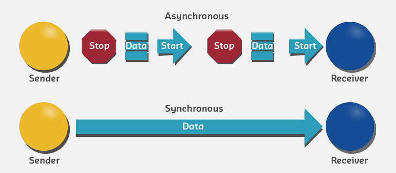
Serial communication protocol is the common protocol used for microcontroller communications. It involves transmitting a series of digital pulses between sender and receiver at a specified data rate, generally divided into synchronous and asynchronous categories.

{
  const container = document.getElementById('kc-mid-5');
  if (container && typeof InlineKnowledgeCheck !== 'undefined') {
    container.innerHTML = '';
    container.appendChild(InlineKnowledgeCheck.create({
      question: "A Zigbee coordinator receives temperature readings from 50 sensors. The MQTT broker topic structure is 'building/floor/room/sensor_type'. What role does topic hierarchy play in the pub/sub pattern?",
      options: [
        {text: "Topics are only for human readability", correct: false, feedback: "Topics serve a functional purpose - they enable selective subscription and message routing, not just readability."},
        {text: "Enables selective subscription and hierarchical message filtering", correct: true, feedback: "Correct! Topic hierarchies allow subscribers to filter messages at different granularities (e.g., 'building/+/+/temperature' for all temps, or 'building/floor1/#' for everything on floor 1), reducing network traffic and processing load."},
        {text: "Required by MQTT protocol specification", correct: false, feedback: "MQTT doesn't require hierarchical topics - flat topics work too. Hierarchy is a design choice for filtering flexibility."},
        {text: "Prevents message delivery delays", correct: false, feedback: "Topic hierarchy doesn't directly affect latency - it's about subscription filtering and logical organization."}
      ],
      difficulty: "medium",
      topic: "pub-sub-patterns"
    }));
  }
}

189.3.1 Asynchronous Serial Communication

⭐⭐ Intermediate

Figure 189.5: Comparison of asynchronous serial communication protocols (UART, RS-232) showing start/stop bits and timing characteristics

In asynchronous serial communication, transmitter and receiver manually agree on the data rate, and each manages timing independently with no common clock. The data rate for the transmitter sending pulses must be the same as the receiver listening for pulses.

189.3.1.1 Required Agreement Parameters

The transmitter and receiver must agree on: - Data rate (baud rate) - Voltage level corresponding to 1 bit or 0 bit - Signal interpretation: High voltage = 1 and low voltage = 0, or inverted

189.3.1.2 Example: 9600 bps Communication

1. Both transmitter and receiver agree on voltage level interpretation for 1 bit and 0 bit
2. Both ends require a common ground connection to measure voltage with same reference point
3. Wire connection for transmission from sender to receiver
4. Wire connection for transmission from receiver to sender

When communication is established with agreed data rate (9600 bps), the receiver reads voltage constantly on the receiving wire and interprets it every 1/9600th of a second.

189.3.1.3 Voltage Levels

Generally, in most microcontrollers: - High voltage (+5V or +3.3V) represents 1 bit - Low voltage (0V) represents 0 bit

At the end of data transmission, the receiver rebuilds the original message using the interpreted bits from voltage levels.

189.3.1.4 Common Asynchronous Protocols

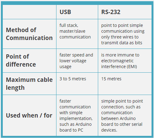
RS-232: - Long-established standard - ±12V signal levels - Long cable runs (up to 15 meters) - Common in industrial equipment

USB (Universal Serial Bus): - High-speed asynchronous serial - Host-device architecture - Power delivery capability - Hot-pluggable

%%{init: {'theme': 'base', 'themeVariables': { 'primaryColor': '#2C3E50', 'primaryTextColor': '#fff', 'primaryBorderColor': '#16A085', 'lineColor': '#16A085', 'secondaryColor': '#E67E22', 'tertiaryColor': '#7F8C8D'}}}%%
graph TB
    subgraph "I2C"
        I2C_Pins["2 Pins<br/>(SDA, SCL)"]
        I2C_Speed["Speed:<br/>100-400 kbps"]
        I2C_Devices["Multiple devices<br/>(127 max)"]
    end

    subgraph "SPI"
        SPI_Pins["4+ Pins<br/>(MISO, MOSI,<br/>SCK, CS)"]
        SPI_Speed["Speed:<br/>1-100 Mbps"]
        SPI_Devices["One device<br/>per CS line"]
    end

    subgraph "UART"
        UART_Pins["2 Pins<br/>(TX, RX)"]
        UART_Speed["Speed:<br/>9600-115200 bps"]
        UART_Devices["Point-to-point<br/>(1 device)"]
    end

    Choose{Choose<br/>Protocol}
    Choose --> |Many sensors| I2C
    Choose --> |High speed| SPI
    Choose --> |Simple serial| UART

    style I2C fill:#16A085,stroke:#2C3E50,color:#fff
    style SPI fill:#E67E22,stroke:#2C3E50,color:#fff
    style UART fill:#2C3E50,stroke:#16A085,color:#fff

Figure 189.6: Serial Protocol Selection: I2C, SPI, and UART Comparison

%%{init: {'theme': 'base', 'themeVariables': { 'primaryColor': '#2C3E50', 'primaryTextColor': '#fff', 'primaryBorderColor': '#16A085', 'lineColor': '#16A085', 'secondaryColor': '#E67E22', 'tertiaryColor': '#7F8C8D'}}}%%
graph TB
    subgraph Application["Application Layer"]
        APP[IoT Application<br/>Sensor reading, data logging]
    end

    subgraph Driver["Driver Layer"]
        I2C_DRV[I2C Driver<br/>Address-based]
        SPI_DRV[SPI Driver<br/>CS-based]
        UART_DRV[UART Driver<br/>Point-to-point]
    end

    subgraph Physical["Physical Layer"]
        I2C_PHY[I2C Bus<br/>2 wires: SDA + SCL<br/>Open-drain, pull-ups]
        SPI_PHY[SPI Bus<br/>4 wires: MOSI MISO SCK CS<br/>Push-pull]
        UART_PHY[UART<br/>2 wires: TX + RX<br/>Async, no clock]
    end

    subgraph Devices["Connected Devices"]
        I2C_DEV[127 devices max<br/>Each has address]
        SPI_DEV[1 per CS line<br/>Full duplex]
        UART_DEV[1 device only<br/>Bidirectional]
    end

    APP --> I2C_DRV
    APP --> SPI_DRV
    APP --> UART_DRV

    I2C_DRV --> I2C_PHY
    SPI_DRV --> SPI_PHY
    UART_DRV --> UART_PHY

    I2C_PHY --> I2C_DEV
    SPI_PHY --> SPI_DEV
    UART_PHY --> UART_DEV

    style Application fill:#2C3E50,color:#fff
    style Driver fill:#E67E22,color:#fff
    style Physical fill:#16A085,color:#fff
    style Devices fill:#7F8C8D,color:#fff

Figure 189.7: Alternative view: Layered architecture showing how applications access sensors through driver abstraction, physical bus characteristics, and device connectivity patterns. This stack view emphasizes the separation of concerns and protocol-specific constraints at each layer.

{fig-alt=“Serial protocol comparison: I2C uses 2 pins (SDA, SCL) at 100-400 kbps supporting multiple devices up to 127 max; SPI uses 4+ pins (MISO, MOSI, SCK, CS) at 1-100 Mbps with one device per chip select; UART uses 2 pins (TX, RX) at 9600-115200 bps for point-to-point one device communication - choose I2C for many sensors, SPI for high speed, UART for simple serial”}

{
  const container = document.getElementById('kc-mid-6');
  if (container && typeof InlineKnowledgeCheck !== 'undefined') {
    container.innerHTML = '';
    container.appendChild(InlineKnowledgeCheck.create({
      question: "An MQTT broker is configured with QoS 1 (at-least-once delivery). A subscriber disconnects during message delivery. What happens to undelivered messages?",
      options: [
        {text: "Messages are immediately discarded", correct: false, feedback: "QoS 1 guarantees at-least-once delivery - the broker stores unacknowledged messages for retry."},
        {text: "Broker queues messages and retries when subscriber reconnects", correct: true, feedback: "Correct! With QoS 1, the broker maintains a session and queues undelivered messages. When the subscriber reconnects (with clean session=false), the broker delivers stored messages to ensure at-least-once delivery."},
        {text: "Messages are sent to a dead-letter queue permanently", correct: false, feedback: "MQTT doesn't have dead-letter queues by default - QoS 1 retries until acknowledged or session expires."},
        {text: "The publisher must resend all messages manually", correct: false, feedback: "QoS 1 handles retries automatically between broker and subscriber - publishers don't manage subscriber delivery."}
      ],
      difficulty: "medium",
      topic: "message-brokers"
    }));
  }
}

189.3.2 Synchronous Serial Communication

⭐⭐ Intermediate

Figure 189.8: Synchronous serial communication diagram showing clock signal coordination between transmitter and receiver for I2C and SPI protocols

Figure 189.9: I2C and SPI protocols comparison - two primary synchronous serial communication protocols for IoT sensor interfacing

In synchronous serial communication, a clocking system manages synchronization between transmitter and receiver. The clock is either: - Embedded as part of the data frame, or - A separate clock wire manages timing during transmission

189.3.2.1 Clock Sharing

All devices in the communication line share the same clock data. With every clock pulse, one bit moves in the line. The clocking system directs devices regarding: - When to listen to incoming bits - When to discard them

This type of communication is used for simpler devices with no internal clock crystal and few memory registers.

189.3.2.2 Common Synchronous Protocols

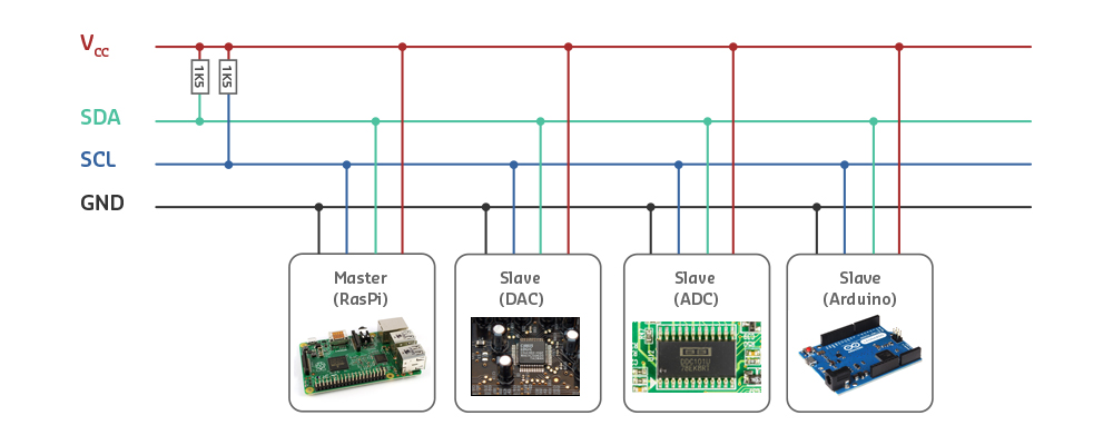
I2C (Inter-Integrated Circuit): - 2-wire bus (SDA: data, SCL: clock) - Multi-master capable - Address-based device selection - Lower speed (100 kHz - 3.4 MHz) - Good for many low-speed peripherals

SPI (Serial Peripheral Interface): - 4-wire bus (MOSI, MISO, SCLK, SS/CS) - Master-slave architecture - Full-duplex communication - Higher speed (up to tens of MHz) - Good for high-speed, few peripherals

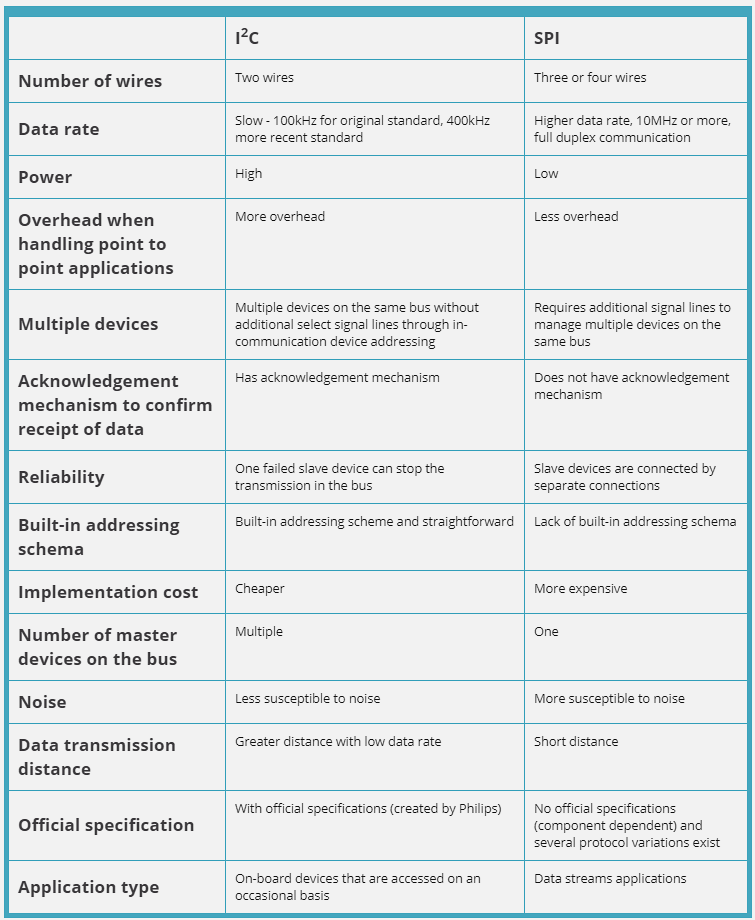
189.3.2.3 I2C vs SPI Comparison

Feature	I2C	SPI
Wires	2 (SDA, SCL)	4 (MOSI, MISO, SCLK, SS)
Topology	Multi-master bus	Master-slave
Speed	100 kHz - 3.4 MHz	Up to 50+ MHz
Device addressing	7 or 10-bit addresses	Chip select pins
Max devices	~127 devices	Limited by CS pins
Complexity	More complex protocol	Simpler protocol
Power	Lower	Slightly higher
Best for	Many slow peripherals	Few fast peripherals
Flow control	Built-in ACK/NACK	No built-in flow control

%%{init: {'theme': 'base', 'themeVariables': { 'primaryColor': '#2C3E50', 'primaryTextColor': '#fff', 'primaryBorderColor': '#16A085', 'lineColor': '#16A085', 'secondaryColor': '#E67E22', 'tertiaryColor': '#7F8C8D'}}}%%
graph TB
    subgraph "I2C"
        I2C_Pins["2 Pins<br/>(SDA, SCL)"]
        I2C_Speed["Speed:<br/>100-400 kbps"]
        I2C_Devices["Multiple devices<br/>(127 max)"]
    end

    subgraph "SPI"
        SPI_Pins["4+ Pins<br/>(MISO, MOSI,<br/>SCK, CS)"]
        SPI_Speed["Speed:<br/>1-100 Mbps"]
        SPI_Devices["One device<br/>per CS line"]
    end

    subgraph "UART"
        UART_Pins["2 Pins<br/>(TX, RX)"]
        UART_Speed["Speed:<br/>9600-115200 bps"]
        UART_Devices["Point-to-point<br/>(1 device)"]
    end

    Choose{Choose<br/>Protocol}
    Choose --> |Many sensors| I2C
    Choose --> |High speed| SPI
    Choose --> |Simple serial| UART

    style I2C fill:#16A085,stroke:#2C3E50,color:#fff
    style SPI fill:#E67E22,stroke:#2C3E50,color:#fff
    style UART fill:#2C3E50,stroke:#16A085,color:#fff

Figure 189.10: Synchronous Serial Protocol Decision Tree: I2C, SPI, and UART

{fig-alt=“Serial protocol comparison: I2C uses 2 pins (SDA, SCL) at 100-400 kbps supporting multiple devices up to 127 max; SPI uses 4+ pins (MISO, MOSI, SCK, CS) at 1-100 Mbps with one device per chip select; UART uses 2 pins (TX, RX) at 9600-115200 bps for point-to-point one device communication - choose I2C for many sensors, SPI for high speed, UART for simple serial”}

189.3.2.4 Selection Guidelines

According to the distinctions between I2C and SPI:

1. I2C is more suitable when:
   • Large number of peripherals needed
   • High data rate NOT required
   • Pin count must be minimized
   • Multi-master capability needed
2. SPI is a good option when:
   • Low power required
   • High speed needed
   • Few peripherals (pin count not constrained)
   • Full-duplex communication needed

Both serial communication protocols are considered stable and robust for embedded applications. The critical part is ensuring both devices on a serial bus are configured to use the exact same protocols.

{
  const container = document.getElementById('kc-mid-7');
  if (container && typeof InlineKnowledgeCheck !== 'undefined') {
    container.innerHTML = '';
    container.appendChild(InlineKnowledgeCheck.create({
      question: "A gateway translates I2C sensor data (binary uint16) to MQTT JSON payloads. The temperature sensor returns raw value 0x0A5A representing 26.50 degrees Celsius. What transformation steps are needed?",
      options: [
        {text: "Just send the hex value as a string in JSON", correct: false, feedback: "Raw hex is not human-readable or useful for analytics - proper translation requires unit conversion and structured formatting."},
        {text: "Convert binary to decimal, apply scaling, format as JSON with metadata", correct: true, feedback: "Correct! Translation involves: 1) Read binary 0x0A5A (2650 decimal), 2) Apply scaling factor (÷100 = 26.50°C), 3) Format as JSON: {\"temperature\": 26.5, \"unit\": \"celsius\", \"timestamp\": \"...\"}."},
        {text: "Send binary directly over MQTT", correct: false, feedback: "While MQTT can carry binary, JSON payloads are standard for interoperability. The key is proper data transformation, not just transport."},
        {text: "Only change the protocol headers, keep data unchanged", correct: false, feedback: "Protocol translation must include data format conversion - I2C binary registers don't map directly to JSON structures."}
      ],
      difficulty: "medium",
      topic: "protocol-translation"
    }));
  }
}

WarningTradeoff: I2C vs SPI for Sensor Communication

Option A: I2C (Inter-Integrated Circuit) - 2-wire bus (SDA + SCL) supporting up to 127 addressed devices at 100kHz-3.4MHz, ideal for connecting many low-speed sensors with minimal GPIO usage.

Option B: SPI (Serial Peripheral Interface) - 4-wire interface (MOSI, MISO, SCLK, CS) offering speeds up to 50+ MHz with dedicated chip select per device, ideal for high-speed peripherals like displays, ADCs, and SD cards.

Decision Factors:

• Choose I2C when: GPIO pins are limited, connecting 5+ sensors (temperature, humidity, IMU), speed under 1 Mbps is acceptable, multi-master capability is needed, or built-in addressing eliminates need for chip select management.

• Choose SPI when: High data rates are required (>1 Mbps), connecting displays or high-speed ADCs, full-duplex communication is needed, fewer than 4 peripherals (CS pins available), or simpler protocol reduces debugging complexity.

• Common pattern: Use I2C for sensor clusters (environmental monitoring) and SPI for high-bandwidth peripherals (SD card logging, TFT display). Many designs use both buses for different device classes.

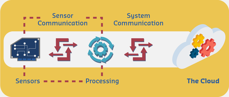
189.4 System Communication

The large amount of data collected by sensors must be transferred to servers on the Cloud for analysis and decision making. Then necessary actions are delivered back from the Cloud to microcontrollers.

Communication between sensors to computer/Cloud is done using communication protocols based on: - Power consumption requirements - Coverage requirements - Data rate requirements - Cost requirements

189.4.1 Ethernet (Wired)

A wired network is the traditional way of connecting devices to the Internet, practical for environments with wired connections, such as smart home systems.

Advantages: - High reliability - High data rates (100 Mbps - 10 Gbps) - No interference - Secure physical connection

Disadvantages: - Requires cable infrastructure - Not suitable for mobile devices - Installation costs

Best for: Smart buildings, industrial IoT, data centers

WarningTradeoff: Wired (Ethernet) vs Wireless Connectivity for IoT

Option A: Wired Ethernet - Physical cable connection providing reliable, high-bandwidth, interference-free communication with Power over Ethernet (PoE) capability for device power.

Option B: Wireless (Wi-Fi, BLE, LoRa, Cellular) - Radio-based connectivity enabling flexible deployment, mobility, and reduced installation costs without cable infrastructure.

Decision Factors:

• Choose Wired when: Devices are stationary in fixed locations, reliability is critical (industrial control, safety systems), high bandwidth is needed (video cameras, data loggers), PoE simplifies power distribution, or security requires physical network isolation.

• Choose Wireless when: Devices are mobile or frequently relocated, cable installation is impractical or expensive, rapid deployment is needed, devices are battery-powered (wired adds power consumption), or legacy buildings lack cabling infrastructure.

• Consider Both when: Backbone infrastructure uses Ethernet while wireless extends to end devices. Gateways bridge Ethernet backhaul with Wi-Fi/BLE sensor networks. This hybrid pattern combines reliability with flexibility.

{
  const container = document.getElementById('kc-mid-8');
  if (container && typeof InlineKnowledgeCheck !== 'undefined') {
    container.innerHTML = '';
    container.appendChild(InlineKnowledgeCheck.create({
      question: "A cloud platform uses Apache Kafka as a message broker for IoT data. Unlike MQTT, Kafka stores messages in partitioned logs. What advantage does this provide for IoT analytics?",
      options: [
        {text: "Lower latency for real-time alerts", correct: false, feedback: "Kafka's log-based storage actually adds slight latency compared to pure pub/sub - its advantage is elsewhere."},
        {text: "Message replay capability for historical analysis and reprocessing", correct: true, feedback: "Correct! Kafka's persistent, ordered log allows consumers to replay messages from any offset - enabling historical analysis, debugging, reprocessing after code fixes, and multiple independent consumers reading the same data stream."},
        {text: "Automatic protocol translation", correct: false, feedback: "Kafka doesn't translate protocols automatically - it's a message broker. Protocol translation requires separate gateway components."},
        {text: "Reduced network bandwidth usage", correct: false, feedback: "Kafka's log storage doesn't reduce bandwidth - it enables durability and replay, which may actually increase storage and I/O."}
      ],
      difficulty: "hard",
      topic: "message-brokers"
    }));
  }
}

189.4.2 Wireless Communication

However, in most IoT scenarios, Ethernet technology is not sufficient and some kind of wireless communication must be implemented based on power consumption, data rate, coverage, and cost.

%%{init: {'theme': 'base', 'themeVariables': { 'primaryColor': '#2C3E50', 'primaryTextColor': '#fff', 'primaryBorderColor': '#16A085', 'lineColor': '#16A085', 'secondaryColor': '#E67E22', 'tertiaryColor': '#7F8C8D', 'fontSize': '11px'}}}%%
graph TB
    subgraph Short["Short Range (< 100m)"]
        Wi-Fi["Wi-Fi<br/>Speed: 150+ Mbps<br/>Power: High<br/>Cost: Low"]
        BLE["BLE<br/>Speed: 2 Mbps<br/>Power: Very Low<br/>Cost: Very Low"]
        Zigbee["Zigbee<br/>Speed: 250 kbps<br/>Power: Low<br/>Cost: Low"]
    end

    subgraph Long["Long Range (> 1 km)"]
        LoRa["LoRa/LoRaWAN<br/>Speed: 50 kbps<br/>Power: Very Low<br/>Range: 15 km"]
        Cellular["Cellular (LTE-M/NB-IoT)<br/>Speed: 1 Mbps<br/>Power: Medium<br/>Range: Wide Area"]
        Sigfox["Sigfox<br/>Speed: 100 bps<br/>Power: Ultra Low<br/>Range: 40 km"]
    end

    Decision{Select Based On}
    Decision -->|High bandwidth| Wi-Fi
    Decision -->|Battery devices| BLE
    Decision -->|Mesh needed| Zigbee
    Decision -->|Remote sensors| LoRa
    Decision -->|Mobile assets| Cellular
    Decision -->|Simple telemetry| Sigfox

    style Short fill:#16A085,stroke:#2C3E50,color:#fff
    style Long fill:#E67E22,stroke:#2C3E50,color:#fff

Figure 189.11: Wireless Protocol Selection for IoT: Short-range protocols (Wi-Fi, BLE, Zigbee) suit indoor and dense deployments; long-range protocols (LoRa, Cellular, Sigfox) enable remote sensing and wide-area coverage.

{
  const container = document.getElementById('kc-mid-9');
  if (container && typeof InlineKnowledgeCheck !== 'undefined') {
    container.innerHTML = '';
    container.appendChild(InlineKnowledgeCheck.create({
      question: "An IoT system uses RabbitMQ as a message queue between edge gateways and cloud processing. Messages have a TTL (time-to-live) of 5 minutes. What happens to sensor readings if the cloud consumer is down for 10 minutes?",
      options: [
        {text: "Messages wait indefinitely until consumer returns", correct: false, feedback: "With TTL configured, messages expire after 5 minutes - they don't wait indefinitely."},
        {text: "Expired messages are discarded or routed to a dead-letter queue", correct: true, feedback: "Correct! Messages exceeding TTL are either discarded or, if configured, routed to a dead-letter exchange/queue for later analysis. This prevents queue buildup but may cause data loss if the consumer is down too long."},
        {text: "RabbitMQ automatically extends the TTL during outages", correct: false, feedback: "TTL is strictly enforced - RabbitMQ doesn't adjust it based on consumer availability."},
        {text: "The gateway stops sending new messages", correct: false, feedback: "Gateways typically don't know about queue TTL expiry - they continue publishing. The queue handles message lifecycle independently."}
      ],
      difficulty: "medium",
      topic: "message-queues"
    }));
  }
}

189.5 Summary

This chapter covered deep dive into sensor-to-microcontroller protocols including i2c, spi, uart, and system communication methods.

Key Takeaways: - Protocol bridging requires understanding timing semantics, not just message translation - Gateway processor requirements depend on edge processing complexity - Different protocols (I2C, SPI, UART, MQTT) have fundamentally different characteristics - Effective gateways implement buffering, state management, and data transformation

189.6 Related Chapters

• Protocol Bridging Overview - Index of all protocol bridging topics
• Previous: Protocol Bridging Fundamentals
• Next: Real-World Gateway Examples

189.7 What’s Next

Continue to Real-World Gateway Examples to learn about study real-world gateway architectures and protocol translation engine designs with practical implementation patterns.