%% fig-alt: "Decision tree flowchart for selecting ad-hoc routing protocol based on network characteristics. Starts with mobility assessment, branches to traffic pattern and network size considerations, and recommends proactive (DSDV, OLSR) for static networks, reactive (DSR, AODV) for mobile/sparse traffic, or hybrid (ZRP, ZHLS) for large heterogeneous networks. Color-coded outcomes: teal for proactive, orange for reactive, gray for hybrid."
%%{init: {'theme': 'base', 'themeVariables': {'primaryColor': '#2C3E50', 'primaryTextColor': '#fff', 'primaryBorderColor': '#16A085', 'lineColor': '#E67E22', 'secondaryColor': '#7F8C8D', 'tertiaryColor': '#ECF0F1'}}}%%
graph TD
    START[Routing Protocol<br/>Selection]

    START --> Q1{Network<br/>Mobility?}
    Q1 -->|Low<br/>Static| PROACTIVE[Proactive Routing<br/>DSDV, OLSR]
    Q1 -->|High<br/>Mobile| Q2{Traffic<br/>Pattern?}

    Q2 -->|Continuous<br/>Dense| PROACTIVE
    Q2 -->|Bursty<br/>Sparse| REACTIVE[Reactive Routing<br/>DSR, AODV]

    Q1 -->|Medium| Q3{Network<br/>Size?}
    Q3 -->|Small<br/><50 nodes| PROACTIVE
    Q3 -->|Large<br/>>100 nodes| HYBRID[Hybrid Routing<br/>ZRP, ZHLS]
    Q3 -->|Medium<br/>50-100 nodes| Q4{Energy<br/>Critical?}

    Q4 -->|Yes| REACTIVE
    Q4 -->|No| PROACTIVE

    style START fill:#2C3E50,stroke:#16A085,color:#fff
    style PROACTIVE fill:#16A085,stroke:#2C3E50,color:#fff
    style REACTIVE fill:#E67E22,stroke:#2C3E50,color:#fff
    style HYBRID fill:#7F8C8D,stroke:#2C3E50,color:#fff
243 Ad-Hoc Networks: Multi-Hop Routing and Protocols
243.1 Learning Objectives
By the end of this chapter, you will be able to:
- Understand Multi-Hop Routing: Describe how packets traverse multiple nodes to reach distant destinations
- Compare Routing Approaches: Distinguish between proactive, reactive, and hybrid routing strategies
- Analyze Trade-offs: Evaluate latency vs overhead, energy vs performance trade-offs
- Select Appropriate Protocols: Choose the right routing approach based on network characteristics
- Interpret Routing Metrics: Understand route discovery latency, overhead, scalability, and energy efficiency
243.2 Prerequisites
Before diving into this chapter, you should be familiar with:
- Ad-Hoc Networks: Core Concepts: Understanding what ad-hoc networks are and their key characteristics
- Multi-Hop Fundamentals: Basic concepts of multi-hop communication
- Routing Fundamentals: General routing concepts
243.3 Multi-Hop Routing Fundamentals
⭐⭐ Intermediate
243.3.1 Why Multi-Hop?
Wireless range limitations necessitate multi-hop communication:
- Range: Low-power radios (BLE, Zigbee) reach 10-100m; coverage areas often span kilometers
- Obstacles: Buildings, terrain, foliage block direct line-of-sight
- Energy: Transmit power scales with distance² (Friis equation); short hops conserve battery
- Interference: Lower power reduces interference with neighbors
243.3.2 Multi-Hop Path Visualization
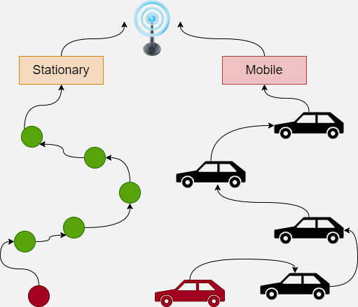
243.3.3 Routing Challenges
Key routing challenges in ad-hoc networks:
- Dynamic Topology: Node mobility, failures, and new joins invalidate routes
- Limited Resources: Battery power, memory, and processing constrain routing overhead
- Unreliable Links: Wireless channels experience fading, interference, and packet loss
- Scalability: Routing table size and update overhead grow with network size
- Loop Prevention: Stale routes can cause forwarding loops and packet storms
243.4 Routing Protocol Categories
⭐⭐⭐ Advanced
243.4.1 Proactive (Table-Driven) Routing
Concept: Nodes maintain routes to all destinations at all times, even before packets need sending.
How It Works:
- Periodic route advertisements (every 5-30 seconds)
- Every node builds complete routing table
- Route available immediately when packet arrives
Examples: DSDV (Destination-Sequenced Distance Vector), OLSR (Optimized Link State Routing)
Trade-offs:
- Pros: Low latency (routes pre-computed), simple forwarding logic
- Cons: High overhead (constant updates), wastes energy when traffic is sparse
Best For: Dense, relatively static networks with continuous traffic
243.4.2 Reactive (On-Demand) Routing
Concept: Routes discovered only when needed; no periodic updates.
How It Works:
- Source floods network with Route Request (RREQ)
- Destination replies with Route Reply (RREP)
- Route cached until link breaks
Examples: DSR (Dynamic Source Routing), AODV (Ad-hoc On-Demand Distance Vector)
Trade-offs:
- Pros: Low overhead (no periodic updates), scales better for sparse traffic
- Cons: High initial latency (route discovery delay), flooding overhead for RREQ
Best For: Sparse, mobile networks with bursty traffic
243.4.3 Hybrid Routing
Concept: Combines proactive (within zones) and reactive (between zones) approaches.
How It Works:
- Proactive routing within local zone (2-3 hop radius)
- Reactive routing for distant destinations
- Zone size adapts to node density and mobility
Examples: ZRP (Zone Routing Protocol), ZHLS (Zone-based Hierarchical Link State)
Trade-offs:
- Pros: Balances latency and overhead, adapts to network conditions
- Cons: Complexity (two protocols), zone size tuning required
Best For: Large, heterogeneous networks with varying traffic patterns
243.5 Routing Protocol Selection
243.5.1 Decision Tree for Protocol Selection
243.5.2 Alternative View: Layered Architecture Design
NoteAlternative View: Layered Architecture Design Hierarchy
This variant shows the same routing protocol selection as a layered architecture - emphasizing how application requirements (top) and network characteristics (bottom) influence routing strategy selection in the middle layer, which then maps to specific protocol implementations:
%%{init: {'theme': 'base', 'themeVariables': {'primaryColor': '#2C3E50', 'primaryTextColor': '#fff', 'primaryBorderColor': '#16A085', 'lineColor': '#E67E22', 'secondaryColor': '#7F8C8D', 'tertiaryColor': '#ECF0F1'}}}%%
graph TB
    subgraph AppLayer["Application Requirements"]
        REQ1[Latency Tolerance]
        REQ2[Traffic Pattern]
        REQ3[Reliability Needs]
    end

    subgraph RouteLayer["Routing Strategy Selection"]
        direction LR
        PROACT[PROACTIVE<br/>Continuous tables<br/>Low latency]
        REACT[REACTIVE<br/>On-demand discovery<br/>Low overhead]
        HYBRID[HYBRID<br/>Zone-based<br/>Balanced]
    end

    subgraph ProtoLayer["Protocol Implementation"]
        DSDV[DSDV<br/>Sequence numbers]
        OLSR[OLSR<br/>MPR optimization]
        DSR[DSR<br/>Source routing]
        AODV[AODV<br/>Hop-by-hop]
        ZRP[ZRP<br/>IARP + IERP]
    end

    subgraph NetLayer["Network Characteristics"]
        NODES[Node Count]
        MOBIL[Mobility Level]
        ENERGY[Energy Budget]
    end

    REQ1 --> PROACT
    REQ2 --> REACT
    REQ3 --> HYBRID

    PROACT --> DSDV
    PROACT --> OLSR
    REACT --> DSR
    REACT --> AODV
    HYBRID --> ZRP

    NODES --> RouteLayer
    MOBIL --> RouteLayer
    ENERGY --> RouteLayer

    style AppLayer fill:#E67E22,color:#fff
    style RouteLayer fill:#2C3E50,color:#fff
    style ProtoLayer fill:#16A085,color:#fff
    style NetLayer fill:#7F8C8D,color:#fff
243.5.3 Alternative View: Operational Comparison
NoteAlternative View: Proactive vs Reactive Operational Comparison
This variant shows the same routing approaches as a side-by-side comparison - emphasizing the operational differences between proactive and reactive routing strategies and their trade-offs:
%%{init: {'theme': 'base', 'themeVariables': {'primaryColor': '#2C3E50', 'primaryTextColor': '#fff', 'primaryBorderColor': '#16A085', 'lineColor': '#E67E22', 'secondaryColor': '#7F8C8D'}}}%%
graph TB
    subgraph Proactive["PROACTIVE ROUTING (DSDV/OLSR)"]
        direction TB
        P_IDLE[Idle Period]
        P_UPDATE[Periodic Updates<br/>Every 15-30 sec]
        P_TABLE[Full Routing Table<br/>Routes to ALL nodes]
        P_SEND[Data Ready to Send]
        P_FWD[Immediate Forward<br/>No discovery delay]

        P_IDLE --> P_UPDATE
        P_UPDATE --> P_TABLE
        P_TABLE --> P_UPDATE
        P_SEND --> P_FWD

        P_PRO[Pros: Low latency]
        P_CON[Cons: High overhead<br/>even when idle]
    end

    subgraph Reactive["REACTIVE ROUTING (DSR/AODV)"]
        direction TB
        R_IDLE[Idle Period<br/>No updates]
        R_SEND[Data Ready to Send]
        R_RREQ[Route Request<br/>Flood network]
        R_WAIT[Wait for Reply<br/>Discovery delay]
        R_FWD[Forward Data<br/>Cache route]

        R_IDLE -.-> R_SEND
        R_SEND --> R_RREQ
        R_RREQ --> R_WAIT
        R_WAIT --> R_FWD

        R_PRO[Pros: Low idle overhead]
        R_CON[Cons: Discovery delay<br/>when sending]
    end

    style P_UPDATE fill:#E67E22,color:#fff
    style P_TABLE fill:#E67E22,color:#fff
    style P_FWD fill:#16A085,color:#fff
    style P_PRO fill:#16A085,color:#fff
    style P_CON fill:#E74C3C,color:#fff
    style R_IDLE fill:#16A085,color:#fff
    style R_RREQ fill:#E67E22,color:#fff
    style R_WAIT fill:#7F8C8D,color:#fff
    style R_FWD fill:#16A085,color:#fff
    style R_PRO fill:#16A085,color:#fff
    style R_CON fill:#E74C3C,color:#fff
243.6 Routing Protocol Comparison Matrix
| Metric | Proactive | Reactive | Hybrid |
|---|---|---|---|
| Route Discovery Latency | Low (immediate) | High (flooding delay) | Medium (zone-dependent) |
| Routing Overhead | High (periodic updates) | Low (on-demand) | Medium (zone updates) |
| Scalability | Poor (O(n²) updates) | Good (O(n) per route) | Good (O(zone size)) |
| Memory Usage | High (full routing table) | Low (active routes only) | Medium (zone + cache) |
| Energy Efficiency | Low (constant overhead) | High (minimal updates) | Medium (zone-dependent) |
| Best Use Case | Dense, static, continuous traffic | Sparse, mobile, bursty traffic | Large, heterogeneous |
243.7 Understanding Multi-Hop Energy Trade-offs
TipUnderstanding Check: Multi-Hop Energy Cost
Scenario: A forest fire detection network has sensors in a line, each 100m apart, extending 1km from gateway. Direct transmission requires 100 mW power but only reaches 100m. Multi-hop transmission uses 10 mW per hop (10x more energy-efficient per hop, but requires multiple hops).
Think about:
- Should the farthest sensor (1km away) use direct long-range transmission or 10-hop multi-hop?
- How many hops make multi-hop more energy-efficient than direct transmission?
- What factors complicate this analysis in real deployments?
Key Insight: Multi-hop is more efficient for distances > 2-3 hops.
Energy comparison:
- Direct transmission (1 km): Requires high-power radio at ~100 mW for 1 km reach. Energy per packet: 100 mW x 10 ms (packet duration) = 1 mJ.
- Multi-hop (10 hops): Each hop: 10 mW x 10 ms = 0.1 mJ. Total 10 hops: 10 x 0.1 mJ = 1 mJ (same as direct!).
Break-even point: Multi-hop becomes efficient when: Hops x E_hop < E_direct. For this example: Hops x 0.1 mJ < 1 mJ -> Hops < 10.
Correction: Radio power scales with distance squared (Friis equation). For 1 km direct transmission, power might be 1000 mW (not 100 mW). Then:
- Direct: 1000 mW x 10 ms = 10 mJ.
- Multi-hop (10 hops): 1 mJ.
Multi-hop is 10x more efficient!
Complicating factors:
- Overhearing cost: Intermediate nodes must stay awake to receive and forward packets. If duty-cycled, forwarding delays accumulate.
- Collision overhead: More transmissions increase collision probability -> retransmissions increase energy.
- Heterogeneous nodes: If intermediate nodes are mains-powered, multi-hop energy cost is externalized.
- Latency: 10 hops x 50 ms/hop = 500 ms latency vs. 10 ms direct.
Design guideline: Multi-hop is energy-efficient for battery-powered networks spanning >500m, but adds latency and complexity. Hybrid approaches use high-power direct links for critical nodes and multi-hop for non-critical sensors.
243.8 Common Pitfalls in Routing Protocol Selection
CautionPitfall: Using Reactive Routing for Continuous Traffic
The mistake: Deploying reactive routing protocols (DSR, AODV) in networks with regular, continuous data flows - such as sensors reporting every 30 seconds.
Why it happens: Teams choose reactive routing because it “saves energy when idle,” without analyzing actual traffic patterns. Marketing materials emphasize on-demand efficiency without mentioning the break-even point.
The fix: Calculate your traffic pattern first. If nodes send data more frequently than once every 2-5 minutes, proactive routing (DSDV, OLSR) typically consumes less energy because route discovery flooding overhead exceeds periodic update cost. Use reactive routing only for sparse, event-driven traffic (alarms, motion detection).
CautionPitfall: Ignoring the Hidden Node Problem
The mistake: Deploying ad-hoc networks without accounting for hidden terminals - nodes that cannot hear each other but interfere at a common receiver, causing collisions and retransmissions.
Why it happens: Simulation tools often use simplified propagation models where “in range” means “can communicate.” Real deployments have asymmetric links, obstacles, and interference patterns that create hidden node scenarios invisible during testing.
The fix: Enable RTS/CTS (Request-to-Send/Clear-to-Send) for networks with >10 nodes or irregular topologies. Use site surveys to identify hidden node pairs. Consider carrier sense threshold tuning. Budget for 20-30% more retransmissions than simulations predict.
CautionPitfall: Flat Routing in Large Networks
The mistake: Using flat routing protocols (where all nodes are equal peers) in networks exceeding 100-150 nodes, leading to routing table explosion and control message flooding.
Why it happens: Initial deployments work fine at 20-50 nodes. As the network grows organically, teams don’t re-evaluate routing architecture. The scalability wall hits suddenly - network performance degrades exponentially, not linearly.
The fix: Design for 3-5x your initial node count from day one. For networks expecting >100 nodes, use hierarchical routing (cluster-based like LEACH) or hybrid approaches (ZRP). Monitor routing table sizes and control message ratios - if control traffic exceeds 15% of total bandwidth, it’s time to restructure.
243.9 Summary
Multi-hop routing is the backbone of ad-hoc networks, enabling communication across distances far beyond single-hop radio range. This chapter covered the three fundamental routing paradigms and their trade-offs.
243.9.1 Key Takeaways
Multi-Hop Necessity: Wireless range limitations (10-100m for low-power radios) require multi-hop routing to cover deployment areas spanning hundreds of meters to kilometers.
Three Routing Paradigms:
- Proactive: Maintains routes to all destinations continuously (low latency, high overhead)
- Reactive: Discovers routes on-demand (low overhead, high initial latency)
- Hybrid: Combines proactive (within zones) and reactive (between zones) for optimal trade-offs
Critical Trade-Offs:
- Latency vs Overhead: Proactive routing offers immediate forwarding but wastes energy on unused routes
- Energy vs Performance: Multi-hop conserves transmit power but adds forwarding overhead at intermediate nodes
- Scalability vs Simplicity: Flat routing is simple but doesn’t scale beyond 100-200 nodes
Protocol Selection Guidelines:
- Use proactive routing when: Network is small (<50 nodes), relatively static, and has continuous traffic patterns
- Use reactive routing when: Network is large, mobile, energy-constrained, and has bursty or sparse traffic
- Use hybrid routing when: Network exceeds 100 nodes with heterogeneous mobility and traffic patterns
Energy Considerations: Multi-hop routing distributes energy consumption across nodes, preventing “energy holes” near the gateway.
243.10 What’s Next
Continue your learning with:
- Ad-Hoc Networks: Applications and Practice: Explore real-world applications, worked examples, and test your knowledge with quizzes
243.10.1 Deep Dive into Specific Protocols
- Ad-hoc Routing: Proactive (DSDV): Learn how Destination-Sequenced Distance Vector maintains loop-free routes through sequence numbers
- Ad-hoc Routing: Reactive (DSR): Explore Dynamic Source Routing’s route caching and source routing mechanisms
- Ad-hoc Routing: Hybrid (ZRP): Understand how Zone Routing Protocol balances proactive and reactive approaches