%%{init: {'theme': 'base', 'themeVariables': { 'primaryColor': '#2C3E50', 'primaryTextColor': '#fff', 'primaryBorderColor': '#16A085', 'lineColor': '#16A085', 'secondaryColor': '#E67E22', 'tertiaryColor': '#7F8C8D'}}}%%
graph TB
    A["ROOT A<br/>Rank: 0<br/>Routing Table:<br/>B→B, C→B, D→C<br/>E→B, F→B"]
    B["Node B<br/>Rank: 100<br/>Routing Table:<br/>E→E, F→F"]
    C["Node C<br/>Rank: 100<br/>Routing Table:<br/>D→D"]
    D["Node D<br/>Rank: 200"]
    E["Node E<br/>Rank: 200"]
    F["Node F<br/>Rank: 200"]

    A --> B
    A --> C
    B --> E
    B --> F
    C --> D

    style A fill:#2C3E50,stroke:#16A085,color:#fff,stroke-width:3px
    style B fill:#16A085,stroke:#2C3E50,color:#fff
    style C fill:#16A085,stroke:#2C3E50,color:#fff
    style D fill:#E67E22,stroke:#2C3E50,color:#fff
    style E fill:#E67E22,stroke:#2C3E50,color:#fff
    style F fill:#E67E22,stroke:#2C3E50,color:#fff
709 RPL Routing Modes and Traffic Patterns
709.1 RPL Routing Modes
RPL supports two modes with different memory/performance trade-offs:
709.1.1 Storing Mode
Each node maintains routing table for its sub-DODAG.
{fig-alt=“RPL Storing mode showing distributed routing tables: ROOT maintains routes to all nodes, intermediate nodes B and C maintain routes to their descendants, enabling distributed forwarding decisions”}
How It Works: 1. DAO messages: Nodes advertise reachability to parents 2. Routing tables: Each node stores routes to descendants 3. Packet forwarding: Node looks up destination in table, forwards to appropriate child
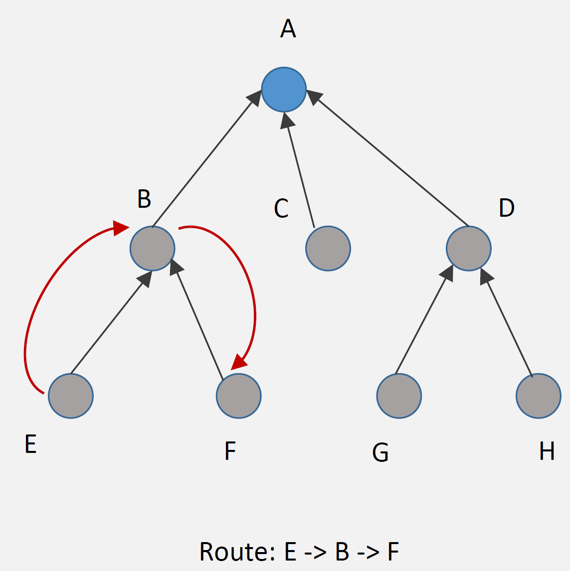
Example Route (E → F):
Step 1: E sends packet to parent B (upward)
Step 2: B checks routing table: "F is my child"
Step 3: B forwards directly to F (downward)

Route: E → B → F (optimal)Advantages: - Efficient routing: Optimal paths (no detour through root) - Low latency: Direct routes between any nodes - Root not bottleneck: Distributed routing decisions
Disadvantages: - Memory overhead: Each node stores routing table - Scalability: Routing tables grow with network size - Updates: DAO messages for every node change
Best For: - Devices with sufficient memory (32+ KB RAM) - Networks requiring low latency - Point-to-point communication common
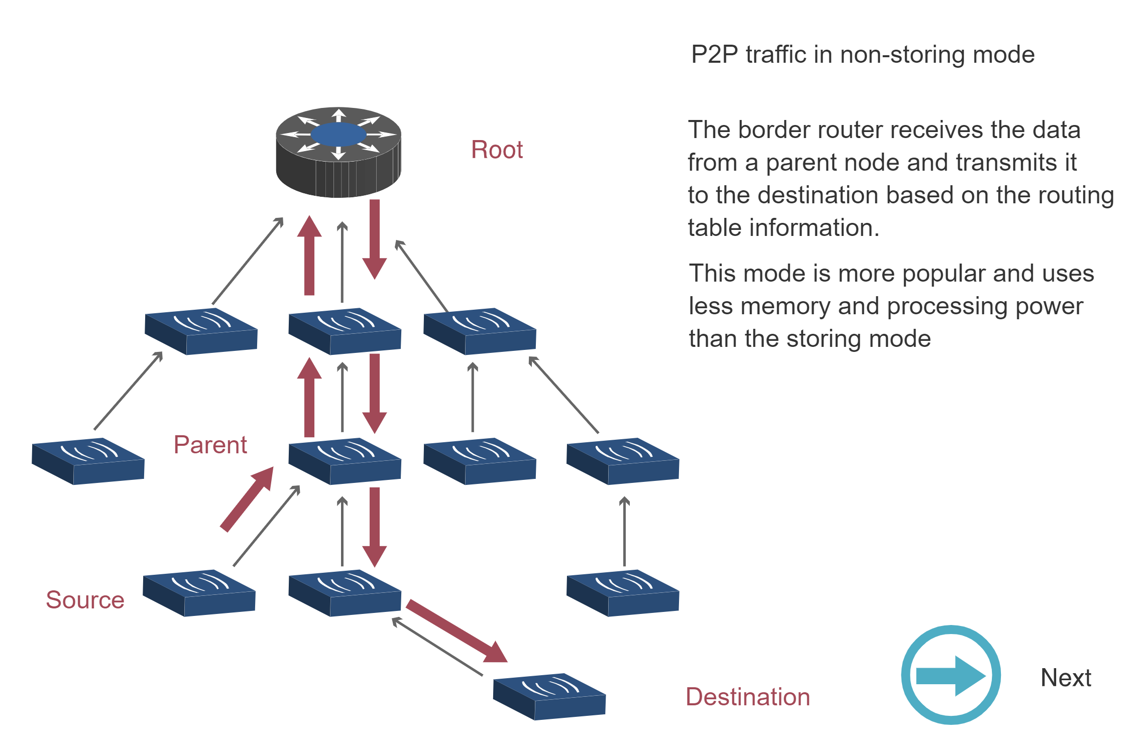
709.1.2 Non-Storing Mode
Only root maintains routing information; exploits source routing.
%%{init: {'theme': 'base', 'themeVariables': { 'primaryColor': '#2C3E50', 'primaryTextColor': '#fff', 'primaryBorderColor': '#16A085', 'lineColor': '#16A085', 'secondaryColor': '#E67E22', 'tertiaryColor': '#7F8C8D'}}}%%
graph TB
    A["ROOT A<br/>Rank: 0<br/>Routing Table:<br/>B→B, C→C, D→C,D<br/>E→B,E, F→B,F<br/>(Complete topology)"]
    B["Node B<br/>Rank: 100<br/>Parent pointer only<br/>(No routing table)"]
    C["Node C<br/>Rank: 100<br/>Parent pointer only<br/>(No routing table)"]
    D["Node D<br/>Rank: 200<br/>Parent: C"]
    E["Node E<br/>Rank: 200<br/>Parent: B"]
    F["Node F<br/>Rank: 200<br/>Parent: B"]

    A --> B
    A --> C
    B --> E
    B --> F
    C --> D

    style A fill:#2C3E50,stroke:#16A085,color:#fff,stroke-width:3px
    style B fill:#16A085,stroke:#2C3E50,color:#fff
    style C fill:#16A085,stroke:#2C3E50,color:#fff
    style D fill:#7F8C8D,stroke:#2C3E50,color:#fff
    style E fill:#7F8C8D,stroke:#2C3E50,color:#fff
    style F fill:#7F8C8D,stroke:#2C3E50,color:#fff
{fig-alt=“RPL Non-Storing mode showing centralized routing at ROOT with complete topology, intermediate nodes maintain only parent pointers, downward routing uses source routing headers from root”}
How It Works: 1. DAO to root: All nodes send DAO directly to root (upward) 2. Root stores all routes: Only root has complete routing table 3. Source routing: Root inserts complete path in packet header 4. Nodes forward: Follow instructions in packet header (no table lookup)
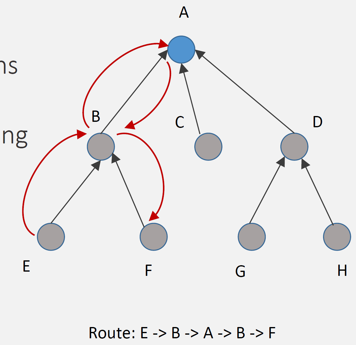
Example Route (E → F):
Step 1: E sends packet to parent B (upward, default route)
Step 2: B forwards to parent A (root) (upward, default route)
Step 3: A (root) checks routing table: "F via B"
Step 4: A inserts source route: [B, F]
Step 5: A sends to B with route in header
Step 6: B forwards to F following route

Route: E → B → A → B → F (via root)Advantages: - Low memory: Nodes don’t store routing tables (just parent) - Simple nodes: Minimal routing logic - Scalability: Network size doesn’t affect node memory
Disadvantages: - Suboptimal routes: All point-to-point traffic via root - Higher latency: Extra hops through root - Root bottleneck: All routing decisions at root - Header overhead: Source route in every packet
Best For: - Resource-constrained devices (< 16 KB RAM) - Primarily many-to-one traffic (sensors → gateway) - Point-to-point communication rare - Large networks (many nodes)
709.1.3 Storing vs Non-Storing Comparison
| Aspect | Storing Mode | Non-Storing Mode |
|---|---|---|
| Routing Table | Distributed (all nodes) | Centralized (root only) |
| Node Memory | Higher (routing table) | Lower (parent pointer only) |
| Route Optimality | Optimal (direct paths) | Suboptimal (via root) |
| Latency | Lower | Higher (extra hops) |
| Root Load | Low | High (all routing decisions) |
| Scalability | Limited by node memory | Limited by root capacity |
| DAO Destination | Parent | Root (through parents) |
| Header Overhead | Low | High (source routing) |
| Best For | Powerful nodes, low latency | Constrained nodes, many-to-one |
TipAlternative View: RPL Mode Selection Decision Tree
This variant provides a practical decision guide for choosing between Storing and Non-Storing modes based on your network characteristics.
%%{init: {'theme': 'base', 'themeVariables': {'primaryColor': '#2C3E50', 'primaryTextColor': '#fff', 'primaryBorderColor': '#16A085', 'lineColor': '#E67E22', 'secondaryColor': '#16A085', 'tertiaryColor': '#E8F6F3', 'fontSize': '10px'}}}%%
flowchart TD
    START["RPL Mode<br/>Selection"] --> Q1{"Primary traffic<br/>pattern?"}

    Q1 -->|"Many-to-One<br/>(sensors→gateway)"| Q2{"Node memory<br/>available?"}
    Q1 -->|"Point-to-Point<br/>(device↔device)"| Q3{"Latency<br/>requirement?"}

    Q2 -->|"< 64KB RAM"| NS1["NON-STORING<br/>━━━━━━━━━━<br/>Memory efficient<br/>Root handles routing<br/>Best: Sensor networks"]
    Q2 -->|"> 64KB RAM"| Q4{"Network size?"}

    Q3 -->|"< 100ms"| ST1["STORING<br/>━━━━━━━━━━<br/>Direct P2P routes<br/>Lower latency<br/>Best: Industrial control"]
    Q3 -->|"> 100ms OK"| NS2["NON-STORING"]

    Q4 -->|"< 200 nodes"| ST2["STORING<br/>━━━━━━━━━━<br/>Optimal paths<br/>Distributed load<br/>Best: Building automation"]
    Q4 -->|"> 200 nodes"| NS3["NON-STORING<br/>━━━━━━━━━━<br/>Scales better<br/>Root manages all"]

    style START fill:#2C3E50,stroke:#16A085,color:#fff
    style Q1 fill:#16A085,stroke:#2C3E50,color:#fff
    style Q2 fill:#16A085,stroke:#2C3E50,color:#fff
    style Q3 fill:#16A085,stroke:#2C3E50,color:#fff
    style Q4 fill:#16A085,stroke:#2C3E50,color:#fff
    style NS1 fill:#E67E22,stroke:#2C3E50,color:#fff
    style NS2 fill:#E67E22,stroke:#2C3E50,color:#fff
    style NS3 fill:#E67E22,stroke:#2C3E50,color:#fff
    style ST1 fill:#2C3E50,stroke:#16A085,color:#fff
    style ST2 fill:#2C3E50,stroke:#16A085,color:#fff
Key Insight: Non-Storing mode is the default choice for resource-constrained sensor networks. Only move to Storing mode when you have both the memory budget AND specific P2P or latency requirements.
NoteAcademic Reference: P2P Traffic Routing Sequence
The following sequence diagrams illustrate how RPL handles point-to-point (P2P) traffic in Non-Storing and Storing modes.
Non-Storing Mode P2P Traffic (Steps 1-3):
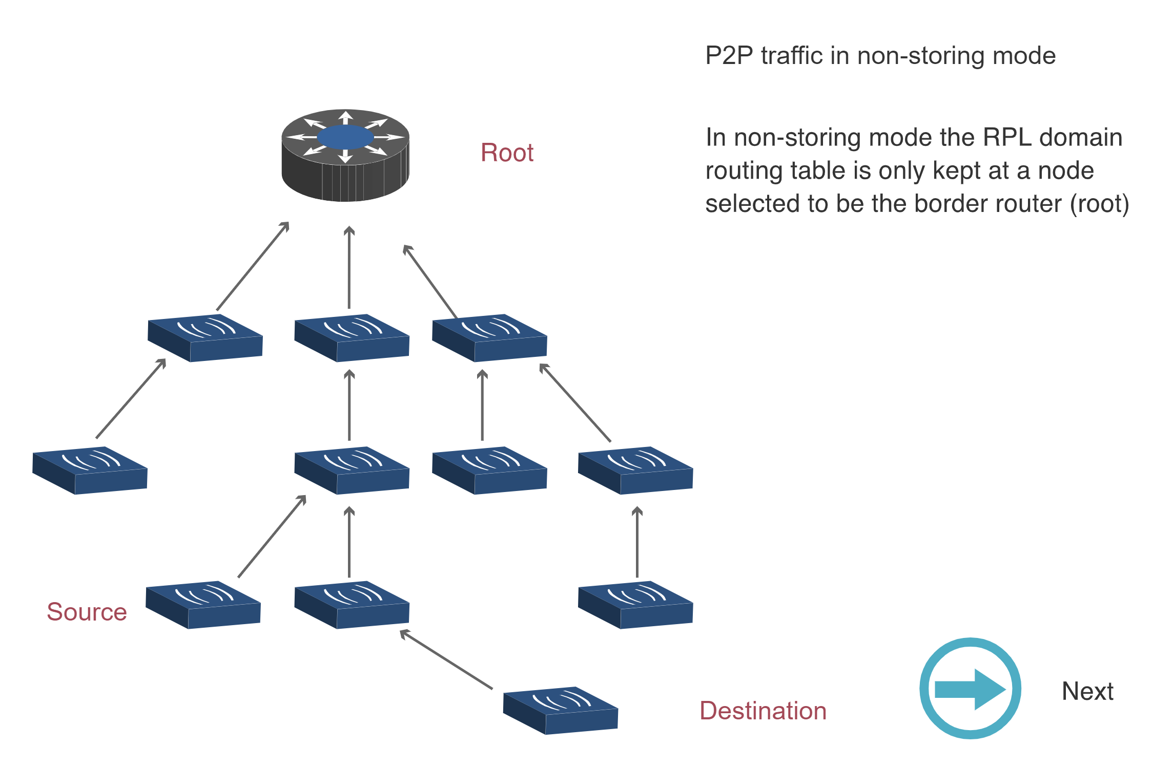
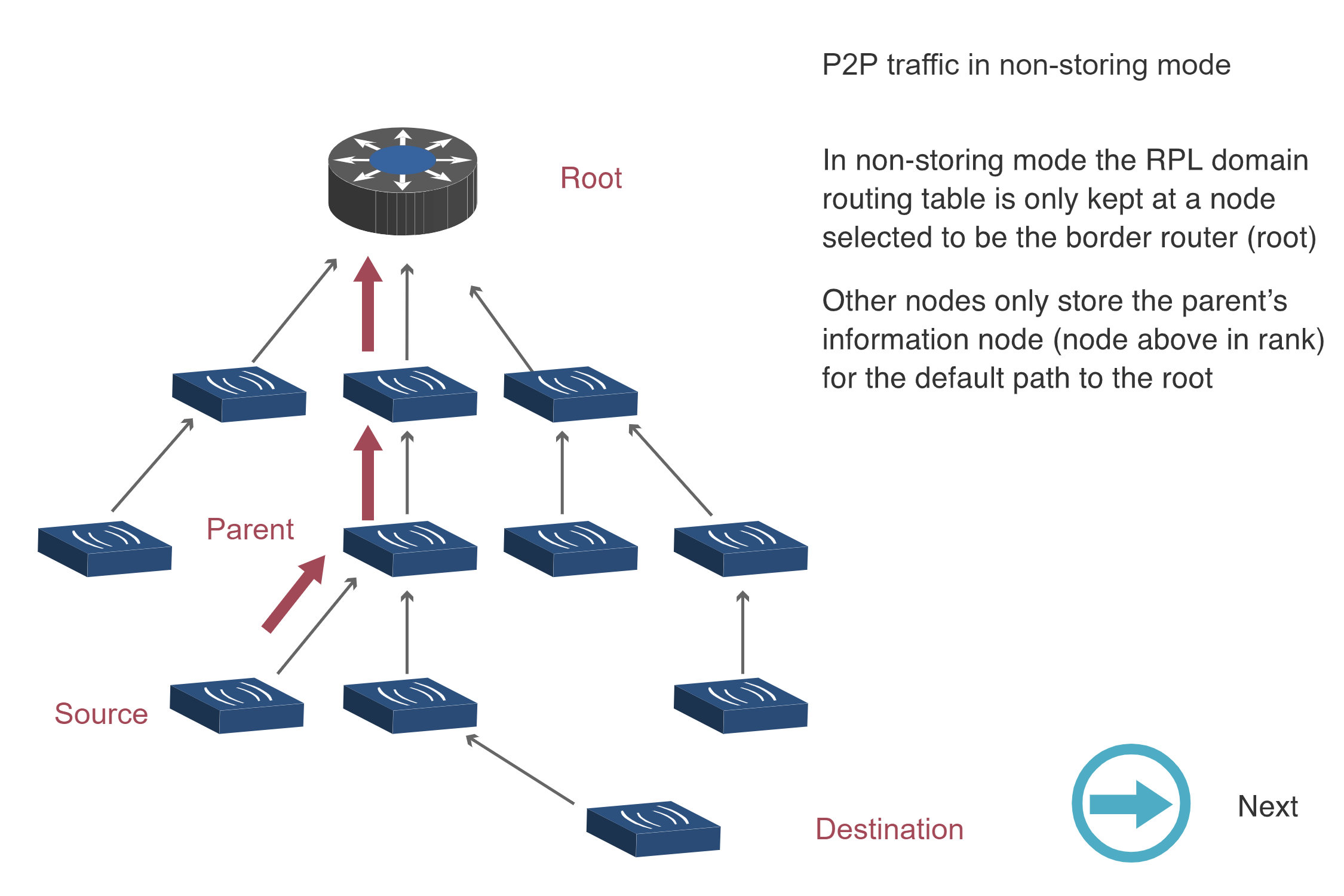
Storing Mode P2P Traffic:
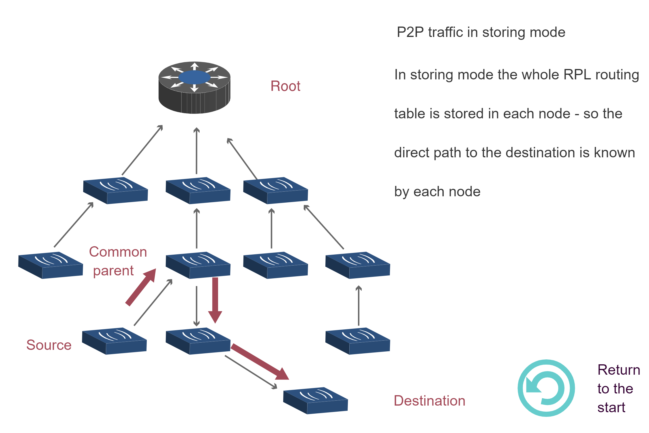
Key Insight: Non-Storing mode requires all P2P traffic to traverse the root (3 diagrams showing upward then downward path), while Storing mode enables direct routing through the nearest common ancestor (1 diagram showing optimized path). This explains why Storing mode has lower latency for P2P traffic despite higher memory requirements.
Source: CP IoT System Design Guide, Chapter 4 - Routing
709.2 RPL Traffic Patterns
RPL optimizes for different traffic directions:
%%{init: {'theme': 'base', 'themeVariables': { 'primaryColor': '#2C3E50', 'primaryTextColor': '#fff', 'primaryBorderColor': '#16A085', 'lineColor': '#16A085', 'secondaryColor': '#E67E22', 'tertiaryColor': '#7F8C8D'}}}%%
graph TB
    subgraph ManyToOne["Many-to-One<br/>(Upward)"]
        S1["Sensor 1"] --> GW1["Gateway"]
        S2["Sensor 2"] --> GW1
        S3["Sensor 3"] --> GW1
        S4["Sensor 4"] --> GW1
    end

    subgraph OneToMany["One-to-Many<br/>(Downward)"]
        GW2["Gateway"] --> A1["Actuator 1"]
        GW2 --> A2["Actuator 2"]
        GW2 --> A3["Actuator 3"]
    end

    subgraph P2P["Point-to-Point"]
        SEN["Sensor"] --> ACT["Actuator"]
    end

    style ManyToOne fill:#16A085,stroke:#2C3E50,color:#fff
    style OneToMany fill:#E67E22,stroke:#2C3E50,color:#fff
    style P2P fill:#7F8C8D,stroke:#2C3E50,color:#fff
    style GW1 fill:#2C3E50,stroke:#16A085,color:#fff
    style GW2 fill:#2C3E50,stroke:#16A085,color:#fff
    style S1 fill:#F8F9FA,stroke:#16A085,color:#2C3E50
    style S2 fill:#F8F9FA,stroke:#16A085,color:#2C3E50
    style S3 fill:#F8F9FA,stroke:#16A085,color:#2C3E50
    style S4 fill:#F8F9FA,stroke:#16A085,color:#2C3E50
    style A1 fill:#F8F9FA,stroke:#E67E22,color:#2C3E50
    style A2 fill:#F8F9FA,stroke:#E67E22,color:#2C3E50
    style A3 fill:#F8F9FA,stroke:#E67E22,color:#2C3E50
    style SEN fill:#F8F9FA,stroke:#7F8C8D,color:#2C3E50
    style ACT fill:#F8F9FA,stroke:#7F8C8D,color:#2C3E50
{fig-alt=“RPL traffic patterns: Many-to-One shows multiple sensors sending to gateway (upward routing), One-to-Many shows gateway sending to multiple actuators (downward), Point-to-Point shows direct sensor to actuator communication”}
709.2.1 Many-to-One (Upward Routing)
Pattern: Many sensors → Single gateway/root
How: - Each node knows parent (from DODAG construction) - Default route: Send to parent (toward root) - No routing table needed (upward)
Example: Temperature sensors reporting to cloud
Sensor 3 → Node 1 → Root → Internet → Cloud
(Upward along DODAG tree)Optimization: - Most common traffic in IoT (data collection) - Minimal state: Just parent pointer - Efficient: Direct path to root
709.2.2 One-to-Many (Downward Routing)
Pattern: Single controller → Many actuators
How: - Storing mode: Each node has routing table, forwards optimally - Non-storing mode: Root inserts source route, nodes follow
Example: Controller sends “turn off” to all lights
Root → [Multicast or unicast to each light]Modes: - Storing: Root → Node 1 → Light 3 (optimal) - Non-storing: Root inserts route [Node 1, Light 3]
709.2.3 Point-to-Point (P2P)
Pattern: Sensor ↔︎ Actuator (peer-to-peer)
How: - Upward then downward (via common ancestor, often root) - Storing mode: May find shorter path - Non-storing mode: Always via root
Example: Motion sensor triggers light
Storing: Sensor 3 → Node 1 → Light 4 (3 hops, if both under Node 1)
Non-Storing: Sensor 3 → Node 1 → Root → Node 2 → Light 4 (4 hops)
709.3 Hands-On Lab: RPL Network Design
NoteLab Activity: Designing RPL Network for Smart Building
Objective: Design an RPL network and compare Storing vs Non-Storing modes
Scenario: 3-floor office building
Devices: - 1 Border Router (roof, internet connection) - 15 mains-powered sensors (temperature, humidity) - can be routers - 30 battery-powered sensors (door, motion) - end devices - 10 actuators (lights, HVAC) - mains powered
Floor Layout:
Floor 3: BR + 5 mains sensors + 10 battery sensors + 3 actuators
Floor 2: 5 mains sensors + 10 battery sensors + 4 actuators
Floor 1: 5 mains sensors + 10 battery sensors + 3 actuators
709.3.1 Task 1: DODAG Topology Design
Design the DODAG: 1. Place border router (root) 2. Identify routing nodes (mains-powered devices) 3. Draw DODAG showing parent-child relationships 4. Assign RANK values (assume RANK increase = 100 per hop)
Click to see solution
DODAG Design:

RANK Distribution: - BR: RANK 0 - Floor 3 mains sensors: RANK 100-200 - Floor 2 mains sensors: RANK 200-400 - Floor 1 mains sensors: RANK 300-500 - Battery/actuators: RANK based on parent + 100
Routing Nodes: 15 mains-powered sensors (can route for battery devices)
Total Nodes: 1 BR + 15 mains + 30 battery + 10 actuators = 56 devices709.3.2 Task 2: Memory Requirements Comparison
Calculate memory requirements for Storing vs Non-Storing:
Assumptions: - IPv6 address: 16 bytes - Next-hop pointer: 2 bytes - Routing entry: 18 bytes total
Calculate: 1. Memory per node (Storing mode) 2. Memory at root (Non-Storing mode) 3. Memory at leaf nodes (both modes)
Click to see solution
Storing Mode:
Routing Table Size per Node: - Root (BR): All 55 devices reachable - 55 entries × 18 bytes = 990 bytes - Mains sensor (typical, 3 children): - 3 entries × 18 bytes = 54 bytes - Battery sensor/actuator (leaf): - 0 entries (just parent pointer: 2 bytes) = 2 bytes
Total network memory (Storing): - BR: 990 bytes - 15 mains sensors × 54 bytes avg = 810 bytes - 40 battery/actuators × 2 bytes = 80 bytes - Total: ~1,880 bytes distributed across network
Non-Storing Mode:
Routing Table Size: - Root (BR): All 55 devices - 55 entries × 18 bytes = 990 bytes - All other nodes: Just parent pointer - 55 nodes × 2 bytes = 110 bytes
Total network memory (Non-Storing): - BR: 990 bytes - 55 other nodes × 2 bytes = 110 bytes - Total: ~1,100 bytes (mostly at root)
Comparison:
| Mode | Root Memory | Node Memory (avg) | Total Memory |
|---|---|---|---|
| Storing | 990 bytes | 15-54 bytes | 1,880 bytes |
| Non-Storing | 990 bytes | 2 bytes | 1,100 bytes |
709.3.3 Task 3: Traffic Pattern Analysis
Analyze routing for different traffic patterns:
Scenarios: 1. Many-to-One: All battery sensors report temperature every 5 minutes to cloud 2. One-to-Many: Cloud sends firmware update to all sensors 3. Point-to-Point: Motion sensor (Floor 1) triggers light (Floor 3)
For each scenario, calculate: - Average hop count (Storing vs Non-Storing) - Messages per minute - Network load
Click to see solution
Scenario 1: Many-to-One (Sensor → Cloud)
Route (any battery sensor to BR): - Storing: Sensor → Parent (mains) → Parent → … → BR - Average: 2-3 hops (battery→mains, mains→BR, possibly intermediate) - Non-Storing: Same (upward routing identical) - Average: 2-3 hops
Messages: - 30 battery sensors × 12 msgs/hour = 360 msgs/hour = 6 msgs/min
Conclusion: Identical performance (many-to-one is RPL’s strength)
Scenario 2: One-to-Many (Cloud → All Sensors)
Route (BR to any sensor): - Storing: BR → optimal path to sensor - BR has routing table, knows best path - Average: 2-3 hops (BR → mains → battery) - Non-Storing: BR → mains → battery (same path, but source routed) - BR inserts source route - Average: 2-3 hops
Difference: Minimal - Storing: routing table lookup at each hop - Non-Storing: source route in header (extra ~10 bytes overhead)
Messages: 55 devices × 1 update = 55 messages (infrequent)
Conclusion: Non-Storing adds header overhead but same hop count
Scenario 3: Point-to-Point (Floor 1 Sensor → Floor 3 Light)
Route: - Storing Mode: ``` Floor 1 Sensor → Parent (Floor 1 mains) Floor 1 mains checks table: “Floor 3 Light not in my sub-tree” → Forward to parent (Floor 2 mains) Floor 2 mains checks table: “Floor 3 Light not in my sub-tree” → Forward to parent (BR) BR checks table: “Floor 3 Light via Sensor 3-2” → Forward to Sensor 3-2 Sensor 3-2 → Floor 3 Light
Path: F1-Sensor → F1-mains → F2-mains → BR → F3-mains → F3-Light Hops: 5 ```
Non-Storing Mode:
Floor 1 Sensor → Parent → ... → BR (upward, default route)
BR inserts source route: [F3-mains, F3-Light]
BR → F3-mains → F3-Light

Path: F1-Sensor → F1-mains → F2-mains → BR → F3-mains → F3-Light
Hops: 5 (same)
Conclusion: For this topology, same hop count, but: - Storing: Distributed routing decisions (higher memory) - Non-Storing: Centralized at root (source routing overhead)
If topology were flatter (e.g., many sensors directly under BR): - Storing: F1-Sensor → BR → F3-Light (2 hops) - Non-Storing: F1-Sensor → BR → F3-Light (2 hops) - Same performance
Summary:
| Traffic Pattern | Storing Advantage | Non-Storing Advantage |
|---|---|---|
| Many-to-One | None (equal) | None (equal) |
| One-to-Many | None (equal) | Lower node memory |
| Point-to-Point | Can optimize locally | Simpler nodes |
709.4 Quiz: RPL Routing Protocol
NoteQuestion 1: RANK Purpose
What is the primary purpose of RANK in RPL?
- To measure the distance in meters from the root
- To prevent routing loops by defining hierarchical position
- To prioritize packets based on importance
- To encrypt routing information
Click to see answer
Answer: B) To prevent routing loops by defining hierarchical position
Explanation:
RANK Definition: RANK is a scalar value representing a node’s position in the DODAG hierarchy relative to the root.
Primary Purpose: Loop Prevention
How RANK Prevents Loops:
- Root has minimum RANK (typically 0)
- RANK increases as you move away from root
- Upward routing rule: Packets forwarded to nodes with lower RANK
- Parent selection rule: Node cannot choose parent with higher RANK
Loop Prevention Example:

Attempt to create loop:
Node C wants to choose Node A as parent: - Current RANK: 400 - Node A RANK: 100 - ✅ ALLOWED (100 < 400, moving toward root)
Node A wants to choose Node C as parent: - Current RANK: 100 - Node C RANK: 400 - ❌ FORBIDDEN (400 > 100, moving away from root = loop!)
Without RANK (e.g., simple hop count):

With RANK:

Option Analysis:
A) Distance in meters ❌ - RANK is not physical distance - RANK is a logical hierarchy in DODAG - Two nodes same distance from root can have different RANKs - Via good link: RANK 100 - Via poor link: RANK 300
B) Prevent routing loops ✅ - Correct: RANK enforces hierarchy - Acyclic property: Prevents cycles in DAG - Rule: Can only route “upward” (decreasing RANK)
C) Prioritize packets ❌ - RANK is for routing, not QoS - Packet prioritization uses different mechanisms: - IPv6 Traffic Class field - RPL can support different objective functions (latency vs energy) - But RANK itself doesn’t prioritize packets
D) Encrypt routing ❌ - RANK is plaintext in DIO messages - Security handled separately: - RPL can use secured mode (RPL Security) - Encryption at link layer (802.15.4 security) - IPsec for end-to-end security - RANK is not a security mechanism
RANK Calculation Factors:
RANK is calculated by objective function, which may consider: - Hop count: Each hop adds fixed amount - ETX: Expected Transmission Count (link quality) - Latency: Time to reach root - Energy: Remaining battery, power consumption - Throughput: Link bandwidth
Example Objective Function (OF0 - Hop Count):
RANK = Parent_RANK + MinHopRankIncrease

MinHopRankIncrease = DEFAULT_MIN_HOP_RANK_INCREASE = 256

Node A (parent: ROOT): RANK = 0 + 256 = 256
Node B (parent: A):    RANK = 256 + 256 = 512
Node C (parent: B):    RANK = 512 + 256 = 768
Example Objective Function (ETX-based):
RANK = Parent_RANK + (ETX × MULTIPLIER)

Good link (ETX = 1.2): RANK increase = 1.2 × 100 = 120
Poor link (ETX = 3.5): RANK increase = 3.5 × 100 = 350

Node might prefer 2 good hops (RANK increase: 240)
over 1 poor hop (RANK increase: 350)