%%{init: {'theme': 'base', 'themeVariables': { 'primaryColor': '#2C3E50', 'primaryTextColor': '#fff', 'primaryBorderColor': '#16A085', 'lineColor': '#16A085', 'secondaryColor': '#E67E22', 'tertiaryColor': '#7F8C8D', 'fontSize': '12px'}}}%%
sequenceDiagram
    participant B as Battery<br/>(2000 mAh)
    participant N as Sensor Node
    participant E as Environment

    Note over B,E: Duty Cycle: Wake every 10 minutes (1% duty cycle)

    rect rgb(44, 62, 80)
    Note over N: SLEEP MODE<br/>10 uA x 10 min<br/>= 0.0017 mAh
    N->>N: Deep Sleep (99% of time)
    end

    rect rgb(22, 160, 133)
    Note over N: WAKE CYCLE<br/>(170ms total)
    E->>N: Temperature reading
    Note over N: Sense: 1mA x 50ms
    N->>N: Process locally
    Note over N: Process: 10mA x 20ms
    end

    alt Threshold exceeded
        rect rgb(230, 126, 34)
        N->>B: Transmit alert!
        Note over N: TX: 30mA x 100ms
        Note over B: Expensive!
        end
    else Normal reading
        Note over N: Skip TX, save energy
    end

    Note over B,E: Result: 2-5 YEAR battery life<br/>(vs 5 days if always awake)
391 WSN Energy Management and Architecture
391.1 Learning Objectives
By the end of this chapter, you will be able to:
- Analyze Energy Consumption: Quantify power consumption across sensing, processing, and transmission activities
- Design Duty Cycling Strategies: Apply sleep scheduling to extend battery life from days to years
- Implement Multi-Hop Routing: Design hierarchical architectures with cluster heads and gateways
- Understand WSN Architecture Tiers: Explain the three-tier architecture from sensor nodes to cloud
- Calculate Energy Tradeoffs: Evaluate transmission power vs. hop count for network lifetime optimization
TipFor Beginners: Energy Management Basics
What is this chapter about? This chapter explains why energy is the most critical constraint in WSN design and how to manage it effectively.
Key Terms:
| Term | Meaning |
|---|---|
| Duty Cycling | Alternating between sleep and wake states |
| Active Power | Energy consumed while sensing/transmitting |
| Sleep Power | Minimal energy consumed while inactive |
| Data Aggregation | Combining multiple readings to reduce transmissions |
Why Energy Matters: - Sensor nodes often use small batteries (AA, coin cell) - Replacing batteries in remote deployments is expensive - A well-designed WSN can operate 5+ years on batteries - Poor design leads to 5-day battery life instead of 5 years
Simple Analogy: Think of your phone battery. If you keep the screen on and use data constantly, it dies in hours. If you turn off notifications and use airplane mode mostly, it lasts days. WSN sensors do the same - sleep most of the time, wake briefly to sense and transmit.
391.2 The Energy Challenge: Why It Matters
The #1 constraint in WSN design is energy. Consider:
| Activity | Power Consumption | Analogy |
|---|---|---|
| Sleeping | ~10 uA | Scout napping |
| Sensing | ~1 mA | Scout looking around |
| Processing | ~10 mA | Scout thinking/calculating |
| Transmitting | ~30-100 mA | Scout shouting to others |
Key insight: Transmitting uses 1000x more power than sleeping!
This is why WSNs use clever tricks: - Duty cycling: Sleep most of the time, wake briefly - Data aggregation: Summarize data locally, send less - Multi-hop: Use nearby nodes instead of shouting far
391.3 Energy Timeline: Duty Cycling in Action
391.3.1 Energy Budget Calculation
Let’s calculate battery life for a typical sensor node:
Scenario: Temperature sensor with 2000 mAh battery
| State | Current | Duration/Hour | Energy/Hour |
|---|---|---|---|
| Sleep | 10 uA | 59.83 min | 0.010 mAh |
| Wake | 1 mA | 0.17 min (6x/hr x 1.7s) | 0.003 mAh |
| Transmit | 30 mA | 0.1 min (6x/hr x 100ms) | 0.003 mAh |
| Total | - | - | 0.016 mAh/hr |
Battery Life = 2000 mAh / 0.016 mAh/hr = 125,000 hours = 14.3 years (theoretical)
In practice, battery self-discharge and environmental factors reduce this to 3-5 years, which is still excellent.
Comparison: Always-On Mode | State | Current | Duration/Hour | Energy/Hour | |——-|———|—————|————-| | Active | 10 mA | 60 min | 10 mAh |
Battery Life = 2000 mAh / 10 mAh/hr = 200 hours = 8 days
Duty cycling extends battery life by 600x!
391.4 WSN Architecture
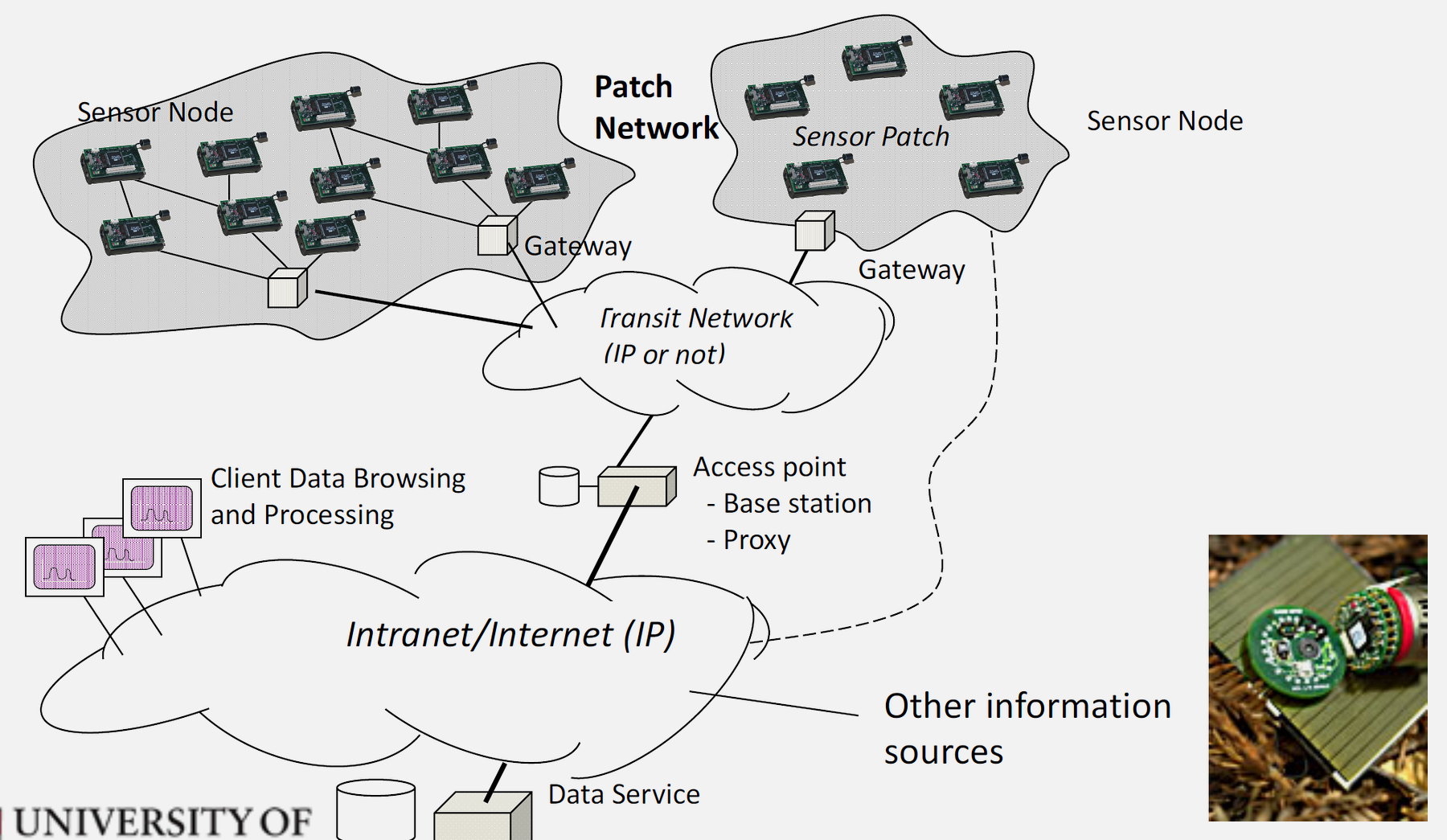
391.4.1 Three-Tier Architecture
Tier 1 - Sensor Nodes: - Collect environmental data through sensors - Perform local processing and filtering - Transmit data to nearby nodes or gateways - Often battery-powered with limited resources
Tier 2 - Gateway/Sink Nodes: - Aggregate data from multiple sensor nodes - Provide protocol translation (e.g., 802.15.4 to Wi-Fi/Ethernet) - Perform edge processing and data fusion - Connect sensor network to external networks
Tier 3 - Backend Systems: - Cloud or on-premise servers - Store and analyze large-scale data - Provide user interfaces and applications - Enable remote management and configuration
391.4.2 Core Characteristics
Distributed Sensing: Multiple sensor nodes deployed across an area provide redundancy, increased coverage, and improved accuracy through collaborative sensing and data fusion.
Wireless Communication: Nodes communicate without physical wiring, enabling deployment in challenging environments and reducing installation costs.
Self-Organization: Networks autonomously configure themselves, adapt to node failures, and optimize routing without centralized coordination.
Resource Constraints: Nodes typically operate under severe constraints in energy, computation, memory, and communication bandwidth.
Application-Specific Design: WSNs are often designed and optimized for specific applications, with hardware and protocols tailored to particular sensing requirements and environmental conditions.
391.5 Multi-Hop Routing Architecture
WSN deployments often require multi-hop communication where sensor nodes relay messages through intermediaries to reach the base station. This diagram illustrates how data flows from edge sensors through cluster heads to the gateway and cloud:
%%{init: {'theme': 'base', 'themeVariables': { 'primaryColor': '#2C3E50', 'primaryTextColor': '#fff', 'primaryBorderColor': '#16A085', 'lineColor': '#16A085', 'secondaryColor': '#E67E22', 'tertiaryColor': '#7F8C8D'}}}%%

graph TB
    subgraph Cloud["Cloud/Backend (Tier 3)"]
        Server[Cloud Server<br/>Analytics & Storage<br/>User Dashboard]
    end

    subgraph Gateway["Gateway Layer (Tier 2)"]
        GW[Gateway/Sink Node<br/>802.15.4 to Wi-Fi/4G<br/>Data Aggregation<br/>Edge Processing]
    end

    subgraph ClusterA["Cluster A"]
        CH1[Cluster Head 1<br/>Relay + Aggregation<br/>Solar Powered]
        S1[Sensor 1<br/>Temperature<br/>Battery: 85%]
        S2[Sensor 2<br/>Humidity<br/>Battery: 92%]
        S3[Sensor 3<br/>Motion<br/>Battery: 78%]

        S1 -->|1 hop| CH1
        S2 -->|1 hop| CH1
        S3 -->|2 hops<br/>via S2| S2
    end

    subgraph ClusterB["Cluster B"]
        CH2[Cluster Head 2<br/>Relay + Aggregation<br/>Solar Powered]
        S4[Sensor 4<br/>Soil Moisture<br/>Battery: 88%]
        S5[Sensor 5<br/>Light<br/>Battery: 91%]
        S6[Sensor 6<br/>Pressure<br/>Battery: 65%]

        S4 -->|1 hop| CH2
        S5 -->|1 hop| CH2
        S6 -->|2 hops<br/>via S4| S4
    end

    subgraph ClusterC["Cluster C - Remote"]
        S7[Sensor 7<br/>Temperature<br/>Battery: 81%]
        S8[Sensor 8<br/>Humidity<br/>Battery: 73%]

        S7 -->|1 hop| S8
        S8 -->|2 hops<br/>via CH1| CH1
    end

    CH1 -->|Aggregated Data<br/>Zigbee/802.15.4| GW
    CH2 -->|Aggregated Data<br/>Zigbee/802.15.4| GW

    GW -->|Internet<br/>Wi-Fi/4G/Ethernet| Server

    style Server fill:#2C3E50,stroke:#16A085,color:#fff
    style GW fill:#E67E22,stroke:#2C3E50,color:#fff
    style CH1 fill:#E67E22,stroke:#2C3E50,color:#fff
    style CH2 fill:#E67E22,stroke:#2C3E50,color:#fff
    style S1 fill:#16A085,stroke:#2C3E50,color:#fff
    style S2 fill:#16A085,stroke:#2C3E50,color:#fff
    style S3 fill:#16A085,stroke:#2C3E50,color:#fff
    style S4 fill:#16A085,stroke:#2C3E50,color:#fff
    style S5 fill:#16A085,stroke:#2C3E50,color:#fff
    style S6 fill:#16A085,stroke:#2C3E50,color:#fff
    style S7 fill:#16A085,stroke:#2C3E50,color:#fff
    style S8 fill:#16A085,stroke:#2C3E50,color:#fff
391.5.1 Key Architecture Principles
- Hierarchical Organization: Sensor nodes - Cluster heads - Gateway - Cloud
- Multi-Hop Communication: Sensors beyond radio range relay through neighbors (e.g., Sensor 3 uses Sensor 2 as relay)
- Data Aggregation: Cluster heads combine data from multiple sensors, reducing transmissions from 8 individual messages to 2 aggregated messages (75% reduction)
- Energy Heterogeneity: Solar-powered cluster heads handle energy-intensive relay tasks; battery sensors only transmit their own data
- Protocol Translation: Gateway bridges low-power WSN protocols (Zigbee, 802.15.4) with Internet protocols (Wi-Fi, 4G, Ethernet)
- Battery Monitoring: Remote visibility of sensor battery levels enables predictive maintenance before failures occur
391.5.2 Historical Evolution
Early Development (1980s-1990s): WSNs emerged from military applications, particularly the Distributed Sensor Networks (DSN) program initiated by DARPA. Early systems were expensive, power-hungry, and limited in capability.
Technological Advancement (2000s): Miniaturization of electronics, advances in wireless communication, and improvements in energy efficiency enabled widespread commercial adoption. The Berkeley Mote platform became a landmark development in WSN research.
IoT Integration (2010s-Present): WSNs have become integral to IoT architectures, with standardized protocols (IEEE 802.15.4, Zigbee, LoRaWAN), cloud integration, and edge computing capabilities transforming their role from isolated systems to connected components of larger ecosystems.
391.6 Case Studies
NoteCase Study: Intel Precision Agriculture - Vineyard Monitoring
Industry: Agriculture / Precision Farming
Challenge: A 500-hectare California vineyard needed to optimize irrigation and detect disease early. Manual soil sampling (technician walks fields weekly with probes) provided sparse data (50 locations per week) with 5-7 day delays, missing critical irrigation windows and allowing diseases to spread. Initial cloud-connected IoT sensors (Wi-Fi-based) failed within 2 months due to: (1) Wi-Fi range limited to 100m requiring 200+ access points ($80K installation cost), (2) High power consumption (200mA idle) drained batteries in 3-6 weeks, requiring constant maintenance.
Solution: Intel deployed Zigbee-based WSN with 800 sensor nodes: - Sensor Nodes (Edge): 800 wireless soil moisture/temperature sensors with Zigbee radios (15mA active, 1uA sleep) deployed every 50m across vineyard rows - Network Topology: Cluster-tree with 40 cluster heads (solar-powered Raspberry Pi + Zigbee coordinator) aggregating data from 20 sensors each - Gateway (Fog): 4G LTE gateway receives compressed data from cluster heads, runs local analytics (anomaly detection, irrigation zone recommendations) - Cloud: Receives hourly summaries for long-term trend analysis, ML model training for disease prediction
Results: - 3-year battery life: Aggressive duty cycling (1% active, 99% sleep) extended node lifetime from 3-6 weeks (Wi-Fi) to 3+ years (Zigbee with sleep), eliminating weekly battery replacement ($50K/year labor savings) - 97% infrastructure cost reduction: Multi-hop Zigbee mesh required only 40 cluster heads + 1 gateway vs. 200 Wi-Fi access points, reducing upfront costs from $80K to $2.4K - 30% water savings: Spatial resolution (800 sensors vs. 50 manual samples) identified micro-zones with optimal moisture, enabling targeted irrigation that saved 12 million gallons annually ($18K water cost savings) - Early disease detection: Daily monitoring (vs. weekly manual) caught downy mildew 5 days earlier, preventing spread that would have cost $120K in lost crop yield
Lessons Learned: 1. Match protocol to power budget - Wi-Fi (200mA idle) is unsuitable for battery-powered sensors; Zigbee (1uA sleep) enables multi-year operation 2. Multi-hop extends coverage economically - Mesh topology with 100m node spacing covers 500 hectares with minimal infrastructure vs. 200+ Wi-Fi access points 3. Cluster heads solve hotspot problem - Solar-powered cluster heads eliminate battery drain from relay traffic; regular nodes only transmit their own data 4. Spatial density reveals patterns - 800 sensors (1.6 per hectare) revealed irrigation inefficiencies invisible to 50 manual samples (0.1 per hectare) 5. Start with high-ROI metrics - Vineyard prioritized soil moisture (direct irrigation savings) before expanding to disease detection, weather monitoring, and yield prediction
NoteCase Study: City of Copenhagen - Smart Parking & Traffic
Industry: Smart City / Transportation
Challenge: Copenhagen’s 300,000+ vehicles spent 20% of drive time searching for parking, creating congestion (85M EUR annual economic cost), emissions (12,000 tons CO2/year), and frustration. Initial parking sensor pilots using cellular IoT (NB-IoT) faced prohibitive costs: 12,000 parking spots x 8 EUR/month cellular = 1.15M EUR/year recurring fees, plus 150 EUR/sensor for cellular modems vs. 30 EUR for Zigbee sensors.
Solution: Copenhagen deployed LoRaWAN-based WSN for citywide parking and traffic monitoring: - Edge Layer: 12,000 wireless parking sensors (magnetic vehicle detection) + 450 traffic counters (ultrasonic) using LoRa radios transmitting every 15 minutes - Network Architecture: Star topology with 85 LoRaWAN gateways (10-15 km range) covering entire city center (88 km2) - Fog Layer: Gateways aggregate sensor data, perform data validation and filtering, transmit summaries to cloud via Ethernet - Cloud Layer: Real-time parking availability map, historical analytics, predictive occupancy models for event planning
Results: - 95% cost reduction: LoRaWAN eliminated cellular fees (0 EUR vs. 1.15M EUR/year) and reduced sensor hardware costs (30 EUR vs. 150 EUR per sensor = 1.44M EUR savings on 12,000 sensors) - 10-year battery life: LoRa’s ultra-low-power operation (12uA sleep, 15-minute reporting) enables decade-long deployments vs. 2-3 years for cellular sensors - 17% traffic reduction: Real-time parking guidance (mobile app + signage) reduced search time from 20% of trips to 3%, cutting inner-city traffic by 17% during peak hours - 35% parking revenue increase: Dynamic pricing based on real-time occupancy increased revenue from 42M EUR to 57M EUR annually while reducing congestion - Emissions reduction: 17% traffic reduction = 2,000+ tons CO2/year avoided, contributing to Copenhagen’s carbon neutrality goals
Lessons Learned: 1. LPWAN economics enable city-scale deployments - LoRaWAN’s zero-fee connectivity and 30 EUR sensors made 12,000-sensor deployment economically viable; cellular costs would have been prohibitive 2. Battery lifetime determines TCO - 10-year battery life eliminates maintenance (replacing 12,000 batteries every 2 years = 240K EUR/year labor), making WSN practical for infrastructure 3. Gateway placement for urban coverage - 85 LoRaWAN gateways (one per km2) provided 99.2% coverage; strategic placement on tall buildings, light poles maximized range 4. Data aggregation at gateway reduces cloud costs - Gateways filter duplicate readings (same car triggering adjacent sensors), validate data (reject physically impossible transitions), reducing cloud processing by 70% 5. Start with revenue-generating use case - Parking sensors had immediate ROI (15M EUR annual revenue increase > 2.5M EUR deployment cost), funding expansion to air quality, waste, and flood monitoring 6. Multi-application infrastructure - LoRaWAN network deployed for parking now supports 35+ applications (waste bins, air quality, traffic, flooding), amortizing infrastructure costs across use cases
NoteKey Concepts
- Duty Cycling: Alternating between sleep and active states to conserve energy, enabling multi-year battery operation
- Data Aggregation: Combining data from multiple sensors at cluster heads to reduce total network transmissions
- Multi-Hop Routing: Relaying data through intermediate nodes to reach destinations beyond direct radio range
- Three-Tier Architecture: Sensor nodes (edge), gateway/sink (fog), and cloud backend for complete IoT integration
- Energy Heterogeneity: Using solar-powered or mains-powered cluster heads for relay tasks while battery sensors only transmit own data
- Protocol Translation: Gateway bridges low-power WSN protocols (Zigbee, 802.15.4) with Internet protocols (Wi-Fi, cellular)
391.7 Summary
This chapter covered energy management and architecture design for wireless sensor networks:
- Energy is the defining constraint - Transmission uses 1000x more power than sleep, requiring duty cycling strategies
- Duty cycling extends battery life dramatically - 1% duty cycle can transform 8-day battery life to 14+ years
- Three-tier architecture provides clear separation between sensing (edge), aggregation (gateway), and analytics (cloud)
- Multi-hop routing extends network range and enables data aggregation at cluster heads
- Real-world deployments demonstrate 3-10 year battery life and 95%+ cost savings over cellular alternatives
Understanding energy management is essential for designing practical WSN deployments that operate reliably for years without maintenance.
391.8 What’s Next?
Continue your WSN learning journey:
- WSN Applications: Explore node identification, collision avoidance, and real-world application domains
- WSN Energy Management: Deep dive into advanced energy conservation strategies
- WSN Sensor Nodes: Learn about sensor node hardware and capabilities
- WSN Deployment Sizing: Plan WSN deployments with sizing calculations