%%{init: {'theme': 'base', 'themeVariables': {'primaryColor': '#2C3E50', 'primaryTextColor': '#fff', 'primaryBorderColor': '#16A085', 'lineColor': '#16A085', 'secondaryColor': '#E67E22', 'tertiaryColor': '#7F8C8D'}}}%%
graph LR
    subgraph BANDWIDTH["Annual Bandwidth Cost (10KB/day)"]
        direction TB
        B1["BLE: 23 bytes/msg<br/>201 MB/year<br/>$20"]
        B2["LoRaWAN: 27 bytes<br/>237 MB/year<br/>$24"]
        B3["UDP/IPv4: 38 bytes<br/>333 MB/year<br/>$33"]
        B4["TCP/IPv4: 50 bytes<br/>438 MB/year<br/>$44"]
        B5["MQTT/IPv6: 72 bytes<br/>631 MB/year<br/>$63"]
    end

    subgraph BATTERY["Battery Impact"]
        direction TB
        BAT1["BLE: 43% payload<br/>Most efficient<br/>5+ year battery"]
        BAT2["LoRaWAN: 37% payload<br/>Good range trade-off<br/>10+ year battery"]
        BAT3["UDP: 26% payload<br/>Moderate overhead<br/>Needs power source"]
        BAT4["TCP: 20% payload<br/>High overhead<br/>Mains powered"]
        BAT5["MQTT: 14% payload<br/>Worst efficiency<br/>Must be plugged in"]
    end

    B1 --> BAT1
    B2 --> BAT2
    B3 --> BAT3
    B4 --> BAT4
    B5 --> BAT5

    style B1 fill:#16A085,stroke:#2C3E50,stroke-width:2px,color:#fff
    style B2 fill:#16A085,stroke:#2C3E50,stroke-width:2px,color:#fff
    style B3 fill:#E67E22,stroke:#2C3E50,stroke-width:2px,color:#fff
    style B4 fill:#E67E22,stroke:#2C3E50,stroke-width:2px,color:#fff
    style B5 fill:#2C3E50,stroke:#E67E22,stroke-width:2px,color:#fff
    style BAT1 fill:#16A085,stroke:#2C3E50,stroke-width:1px,color:#fff
    style BAT2 fill:#16A085,stroke:#2C3E50,stroke-width:1px,color:#fff
    style BAT3 fill:#E67E22,stroke:#2C3E50,stroke-width:1px,color:#fff
    style BAT4 fill:#E67E22,stroke:#2C3E50,stroke-width:1px,color:#fff
    style BAT5 fill:#2C3E50,stroke:#E67E22,stroke-width:1px,color:#fff
53 Protocol Overhead and Encapsulation
53.1 Learning Objectives
By the end of this chapter, you will be able to:
- Compare protocol overhead: Evaluate header sizes across different IoT protocols
- Understand encapsulation: Explain the “Russian doll” model of protocol layering
- Calculate efficiency: Determine bandwidth costs for different protocol stacks
- Choose protocols: Select appropriate protocols based on overhead constraints
NoteRelated Chapters
Prerequisites (Read These First): - Packet Anatomy - Headers, payloads, and trailers fundamentals - Frame Delimiters and Boundaries - Framing and MTU concepts - Error Detection - Checksums and CRC
Companion Chapters (Packet Structure Series): - Packet Structure Overview - Index of all packet structure topics
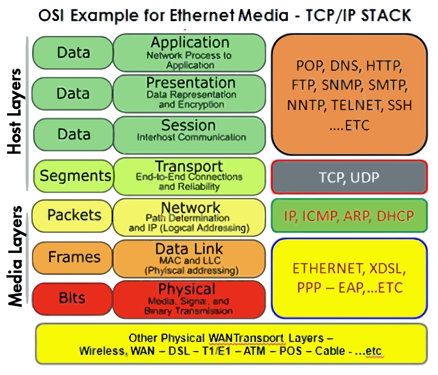
Networking Foundations: - Layered Models - OSI and TCP/IP encapsulation - Transport Protocols - TCP/UDP packet headers
Protocol-Specific Details: - MQTT - MQTT fixed/variable headers - CoAP - CoAP 4-byte header - LoRaWAN - LoRa MAC header - 6LoWPAN - IPv6 header compression
Design & Analysis: - Network Traffic Analysis - Wireshark packet inspection
53.2 Protocol Header Comparison
Different IoT protocols have vastly different header sizes and overhead. Understanding this helps you choose the right protocol for bandwidth-constrained applications.
53.2.1 Real Protocol Headers Compared
Here’s how common IoT protocols stack up when sending a 10-byte sensor payload:
| Protocol | Header Size | Trailer/FCS | Total Overhead | Total Packet | Overhead % |
|---|---|---|---|---|---|
| LoRaWAN | 13 bytes | 4 bytes (MIC) | 17 bytes | 27 bytes | 63% |
| CoAP/UDP/IPv6 | 4+8+40 bytes | - | 52 bytes | 62 bytes | 84% |
| MQTT/TCP/IPv6 | 2+20+40 bytes | - | 62 bytes | 72 bytes | 86% |
| BLE | 10 bytes | 3 bytes (CRC) | 13 bytes | 23 bytes | 57% |
| Zigbee (802.15.4) | 25 bytes | 2 bytes (FCS) | 27 bytes | 37 bytes | 73% |
| TCP/IPv4 | 20+20 bytes | - | 40 bytes | 50 bytes | 80% |
| UDP/IPv4 | 8+20 bytes | - | 28 bytes | 38 bytes | 74% |
Key Insights:
- MQTT over TCP/IPv6: 86% overhead for a 10-byte payload! (72 bytes total)
- LoRaWAN: 63% overhead but optimized for long-range, low-power
- BLE: Best overhead ratio (57%) for short-range applications
- CoAP/UDP: Better than MQTT but still 84% overhead
53.2.2 Real-World Impact
For 1000 sensors sending 10 bytes every hour for a year:
| Protocol | Annual Data Volume | @ $0.10/MB Backhaul Cost |
|---|---|---|
| Raw Data | 88 MB | $8.80 |
| BLE | 201 MB | $20.10 |
| LoRaWAN | 237 MB | $23.70 |
| UDP/IPv4 | 333 MB | $33.30 |
| TCP/IPv4 | 438 MB | $43.80 |
| MQTT/TCP/IPv6 | 631 MB | $63.10 |

53.3 Protocol Encapsulation: The Russian Doll Model
Each protocol layer wraps the data from the layer above, like Russian nesting dolls. Understanding this is key to:
- Reading packet captures in Wireshark - see how protocols nest inside each other
- Calculating MTU and overhead - know why large payloads get fragmented
- Debugging network issues - identify which layer is causing problems
- Designing efficient IoT protocols - minimize unnecessary wrapping
53.3.1 How Encapsulation Works
When you send data through a network, each layer adds its own header (and sometimes trailer) around the data from the layer above:
- Application Layer creates data (e.g., MQTT Publish message)
- Transport Layer wraps it with TCP/UDP header
- Network Layer wraps that with IP header
- Data Link Layer wraps everything with Ethernet header and trailer

%%{init: {'theme': 'base', 'themeVariables': {'primaryColor': '#2C3E50', 'primaryTextColor': '#fff', 'primaryBorderColor': '#16A085', 'lineColor': '#16A085', 'secondaryColor': '#E67E22', 'tertiaryColor': '#7F8C8D'}}}%%
graph LR
    subgraph SENSOR["Temperature Sensor"]
        S1["Read: 23.5C"]
        S2["MQTT Publish<br/>topic/temp"]
    end

    subgraph Wi-Fi["Wi-Fi Chip"]
        W1["Add TCP header<br/>Port 1883"]
        W2["Add IP header<br/>192.168.1.10"]
        W3["Add 802.11 frame<br/>MAC address"]
    end

    subgraph ROUTER["Home Router"]
        R1["Strip 802.11"]
        R2["Add Ethernet"]
        R3["Forward to ISP"]
    end

    subgraph CLOUD["Cloud Broker"]
        C1["Strip headers"]
        C2["Extract MQTT"]
        C3["Store: 23.5C"]
    end

    S1 --> S2
    S2 -->|"2 bytes"| W1
    W1 -->|"+20 bytes"| W2
    W2 -->|"+20 bytes"| W3
    W3 -->|"+34 bytes"| R1
    R1 --> R2 --> R3
    R3 --> C1 --> C2 --> C3

    style S1 fill:#16A085,stroke:#2C3E50,stroke-width:2px,color:#fff
    style S2 fill:#16A085,stroke:#2C3E50,stroke-width:2px,color:#fff
    style W1 fill:#2C3E50,stroke:#16A085,stroke-width:1px,color:#fff
    style W2 fill:#2C3E50,stroke:#16A085,stroke-width:1px,color:#fff
    style W3 fill:#2C3E50,stroke:#16A085,stroke-width:1px,color:#fff
    style R1 fill:#E67E22,stroke:#2C3E50,stroke-width:1px,color:#fff
    style R2 fill:#E67E22,stroke:#2C3E50,stroke-width:1px,color:#fff
    style R3 fill:#E67E22,stroke:#2C3E50,stroke-width:1px,color:#fff
    style C1 fill:#7F8C8D,stroke:#2C3E50,stroke-width:1px,color:#fff
    style C2 fill:#7F8C8D,stroke:#2C3E50,stroke-width:1px,color:#fff
    style C3 fill:#16A085,stroke:#2C3E50,stroke-width:2px,color:#fff
53.3.2 Overhead Calculation Example: Sending 1 Byte of Sensor Data
What happens when you send just 1 byte of temperature data through a standard network stack?
| Layer | Header/Trailer Size | Running Total | Purpose |
|---|---|---|---|
| Application (MQTT) | ~2 bytes header | 3 bytes | MQTT packet type and flags |
| Transport (TCP) | 20 bytes header | 23 bytes | Source/dest ports, sequence numbers, checksums |
| Network (IPv4) | 20 bytes header | 43 bytes | Source/dest IP addresses, TTL, protocol |
| Data Link (Ethernet) | 14+4 bytes header+FCS | 61 bytes | MAC addresses, frame type, error detection |
Result: 1 byte of actual sensor data requires 61 bytes on the wire = 98% overhead!
This is why IoT protocols like CoAP/UDP and 6LoWPAN header compression matter so much for constrained networks.
53.3.3 Protocol Overhead Comparison for IoT
Different protocol stacks have dramatically different overhead. Here’s the minimum packet size for common IoT protocols:
| Protocol Stack | Minimum Packet Size | Overhead for 1 Byte | Best Use Case |
|---|---|---|---|
| Standard HTTP/TCP/IP | ~500+ bytes | 99.8% | NOT suitable for IoT |
| MQTT/TCP/IPv4 | ~62 bytes | 98% | Internet-scale pub/sub |
| CoAP/UDP/IPv4 | ~52 bytes | 98% | Constrained RESTful |
| CoAP/UDP/6LoWPAN | ~16 bytes | 94% | IPv6 over constrained networks |
| MQTT-SN | ~7 bytes | 86% | Sensor networks, UDP-based |
| Raw IEEE 802.15.4 | ~25 bytes | 96% | Low-power wireless (Zigbee, Thread) |
| BLE | ~23 bytes | 96% | Short-range, low-power |
| LoRaWAN | ~21 bytes | 95% | Long-range, low-power (10+ km) |
Key Insights:
- Standard web protocols (HTTP/TCP/IP) waste bandwidth with massive headers
- CoAP over UDP reduces overhead by removing TCP complexity
- 6LoWPAN compression reduces IPv6 headers from 40 bytes to ~2 bytes
- MQTT-SN is optimized for sensor networks (UDP instead of TCP)
- LoRaWAN minimizes overhead while maintaining security (encryption + MIC)
Why This Matters:
- Bandwidth costs: Cellular IoT charges per byte - overhead directly impacts your bill
- Battery life: More data transmitted = more radio time = faster battery drain
- Airtime limits: LoRaWAN has strict duty cycle limits (1% airtime in EU) - overhead counts against your quota
- Network congestion: More overhead = more collisions in shared wireless channels
53.3.4 Practical Encapsulation Example: Wireshark View
When you capture packets with Wireshark, you can literally see the Russian doll unwrapping:
Frame 1: 158 bytes on wire
  Ethernet II, Src: 00:1a:2b:3c:4d:5e, Dst: 00:6f:7e:8d:9c:0b
    - Header: 14 bytes
    - Trailer (FCS): 4 bytes
  Internet Protocol Version 4, Src: 192.168.1.100, Dst: 10.0.0.50
    - Header: 20 bytes
  Transmission Control Protocol, Src Port: 1883, Dst Port: 52341
    - Header: 20 bytes
  MQTT Protocol
    - Fixed Header: 2 bytes
    - Payload: 100 bytes (TEMPERATURE=22.5C)
Reading this capture tells you:
- Total overhead: 14 + 20 + 20 + 2 = 56 bytes (36% of total packet)
- MQTT uses TCP port 1883 (standard MQTT port)
- IP addresses show sensor (192.168.1.100) talking to broker (10.0.0.50)
- MAC addresses identify physical network adapters
- Payload is 100 bytes - the actual sensor data
Understanding encapsulation helps you:
- Debug connectivity issues - which layer is failing?
- Optimize bandwidth - is overhead too high?
- Verify security - is encryption applied at the right layer?
- Calculate MTU - will your packet fit or get fragmented?
TipConnect to Protocol-Specific Chapters
To understand how different IoT protocols handle encapsulation and overhead:
Optimized IoT Protocols: - CoAP Architecture - Lightweight RESTful protocol over UDP - MQTT Overview - Pub/Sub with TCP reliability - 6LoWPAN Fundamentals - IPv6 header compression for constrained networks
Low-Power Wireless: - LoRaWAN Overview - Long-range with minimal overhead - Bluetooth Architecture - BLE protocol stack - Zigbee Architecture - IEEE 802.15.4 frame structure
Network Analysis: - Network Traffic Analysis - Wireshark packet dissection techniques - Layered Models - OSI and TCP/IP encapsulation details - Transport Protocols - TCP vs UDP trade-offs
53.4 Knowledge Check: Protocol Overhead
TipQuiz: LoRaWAN Packet Overhead Analysis
Scenario: You’re deploying 500 soil moisture sensors across a vineyard using LoRaWAN. Each sensor needs to send a 4-byte payload (2 bytes moisture, 2 bytes battery voltage) every 30 minutes. The LoRaWAN protocol adds: - 13-byte header (MHDR, DevAddr, FCtrl, FCnt) - 4-byte trailer (MIC for authentication/integrity)
Your cellular data plan costs $0.10 per MB for the LoRaWAN gateway backhaul.
Think about: 1. What’s the total packet size for each transmission? (Header + Payload + Trailer) 2. What percentage of transmitted data is actual sensor data vs. protocol overhead? 3. How many bytes per sensor per day? How much does backhaul cost per year for 500 sensors?
Key Insights: - Total packet size: 13 + 4 + 4 = 21 bytes per transmission - Overhead ratio: Only 4 bytes out of 21 (19%) is actual data - 81% is protocol overhead! - Daily per sensor: 21 bytes x 48 transmissions/day = 1,008 bytes/day - Annual backhaul: 500 sensors x 1008 bytes x 365 days = 184 MB/year = $18.40/year
Real-world impact: Even with high protocol overhead, LoRaWAN can still be cost-effective for low-bandwidth IoT because messages are tiny. In practice, the bigger differentiator vs Wi-Fi is often power: higher duty cycle and active radio time can shorten battery life and increase maintenance cost.
Understanding packet structure helps you estimate bandwidth costs and choose appropriate protocols for your IoT deployment.
53.5 Scenario-Based Practice
53.6 Additional Knowledge Check
Knowledge Check: Packet Structure Quick Check
Concept: Understanding packet components, framing, and error detection.
A LoRaWAN packet has 13 bytes of header/overhead. If you send 20 bytes of sensor data, what percentage is overhead?
B is correct. Total packet = 13 + 20 = 33 bytes. Overhead percentage = 13/33 = 39.4%. For IoT, overhead is significant - doubling payload to 40 bytes drops overhead to 24.5%. This is why batching sensor readings is efficient.
An IoT device sends temperature readings over UDP. The reading is 23.5C but arrives as 73.5C. Where did the error most likely occur?
D is correct. UDP/IP checksums would detect bit flips (C). If headers were corrupted (A, B), the packet wouldn’t arrive at all. A change from 23.5 to 73.5 (exactly 50C difference) suggests an encoding/decoding mismatch - perhaps degrees Fahrenheit vs Celsius, or an offset error in the application layer.
53.7 Visual Reference Gallery
NoteEncapsulation and Decapsulation (Original Source Figure)
Source: CP IoT System Design Guide, Chapter 4 - Networking Fundamentals
NotePacket Switching Overview (Original Source Figure)
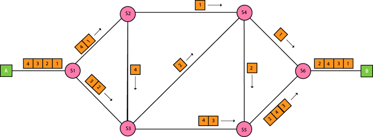
Source: CP IoT System Design Guide, Chapter 4 - Networking Fundamentals
NoteDatagram Structure (Original Source Figure)
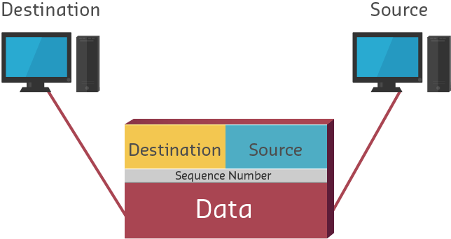
Source: CP IoT System Design Guide, Chapter 4 - Networking Fundamentals
NotePacket Encapsulation (Alternative View)

Packet encapsulation is the process of wrapping data with protocol headers as it descends through the network stack. Each layer adds its own header containing routing, control, and error-checking information. This “Russian doll” structure allows each protocol layer to operate independently while ensuring data reaches its destination correctly. Understanding encapsulation is essential for calculating protocol overhead and debugging network issues with tools like Wireshark.
NotePacket Switching (Alternative View)

Packet switching divides data into discrete packets that travel independently through the network. Unlike circuit switching (dedicated paths), packet switching allows multiple conversations to share network resources efficiently. Each packet contains destination address information enabling routers to forward it along optimal paths. This fundamental networking technique enables the scalable, resilient communication that powers IoT systems from smart homes to industrial networks.
NoteEncapsulation and Decapsulation Process (Alternative View)

The encapsulation/decapsulation process shows the symmetry of network communication. At the sender, each layer adds its header as data descends the stack. At the receiver, each layer removes and processes its header as data ascends. This layered approach enables protocol independence: changes to one layer (e.g., switching from Wi-Fi to Ethernet) don’t require changes to other layers. For IoT developers, understanding this process clarifies how sensor data transforms from application-level readings to physical bits on the wire.
53.8 Summary
Protocol overhead and encapsulation determine IoT system efficiency:
- Protocol Stacking: Each layer adds headers, compounding overhead
- Overhead Impact: Small payloads suffer most - 1 byte can become 61 bytes
- Protocol Choice: BLE/LoRaWAN minimize overhead; TCP/IPv6 maximizes features
- Encapsulation: Russian doll model wraps data at each layer
- Cost Implications: Overhead directly impacts bandwidth costs and battery life
Key Takeaways: - Protocol overhead is significant for small IoT payloads - Choose protocols based on your bandwidth and power constraints - Wireshark reveals encapsulation layers for debugging - 6LoWPAN and header compression reduce IPv6 overhead for constrained networks
53.9 What’s Next
You’ve completed the packet structure series! Continue your learning with:
- Data Formats for IoT - How sensor data gets encoded in the packet payload
- Protocol Selection Framework - Choosing the right protocol for your application
- Network Traffic Analysis - Wireshark packet dissection techniques