652 Layered Models: Labs and Implementation

652.1 Learning Objectives

By the end of this chapter, you will be able to:

Work with MAC Addresses: Read, interpret, and configure hardware addresses on IoT devices
Implement Layer 2 Communication: Use Ethernet and Wi-Fi protocols for local network communication
Analyze Network Frames: Capture and dissect data link layer frames using packet analyzers
Configure ARP: Understand Address Resolution Protocol for IP-to-MAC mapping
Design Local Networks: Plan L2 topologies for IoT deployments with switches and access points
Troubleshoot Connectivity: Diagnose MAC-level issues including duplicate addresses and broadcast storms

652.2 Prerequisites

Before diving into this chapter, you should be familiar with:

Layered Models: Fundamentals: Understanding of the OSI and TCP/IP layered models is essential for grasping how Layer 2 (Data Link) and Layer 3 (Network) work together through encapsulation
Networking Basics for IoT: Basic networking concepts including network topologies, addressing schemes, and protocol fundamentals provide context for MAC and IP addressing
Binary and hexadecimal arithmetic: MAC addresses are 48-bit values represented in hexadecimal, and subnet calculations require binary operations, so comfort with these number systems is important
Command-line basics: Labs use terminal commands (ipconfig, arp, ifconfig) to explore network configuration, so familiarity with command-line interfaces is helpful

652.3 🌱 Getting Started (For Beginners)

For Beginners: Using Labs to Make the OSI Model Concrete

The fundamentals chapter introduced layered models in theory. This chapter shows you what those layers look like on real devices.

As you run the labs (ipconfig, arp, packet captures), always ask:
- Which layer am I looking at right now? (MAC, IP, TCP/UDP, application)
- How does this field relate to the diagrams in layered-models-fundamentals.qmd?
If you cannot run the commands:
- Study the sample outputs and highlight which parts are Layer 2 (MAC) vs Layer 3 (IP).

Helpful mapping while you work:

Layer	Examples in this chapter
L2	MAC addresses, Ethernet frames, ARP table
L3	IPv4 addresses, subnet masks, routing entries
L4	TCP/UDP ports shown in packet captures

If layer boundaries still feel abstract, revisit layered-models-fundamentals.qmd and then use these labs as a “field guide” that ties the conceptual stack to actual commands and packet traces.

Related Chapters

Fundamentals: - Layered Models Fundamentals - OSI/TCP-IP model theory - Layered Network Models - Complete layered model exploration - Networking Basics - Network fundamentals and topologies

Addressing: - Addressing and Subnetting - IP addressing and subnet design - Network Access and Physical - Physical layer protocols

Implementation: - Networking Labs - Additional hands-on exercises - Wired Communication - UART, I2C, SPI protocols

Review: - Layered Models Review - Assessment and comprehensive quiz

Learning: - Simulations Hub - Network protocol simulators and tools

652.4 Data Link Layer: MAC Addressing

⏱️ ~15 min | ⭐⭐⭐ Advanced | 📋 P07.C08.U01

Data link layer diagram showing its position between network and physical layers, with responsibilities including framing, addressing (MAC), error detection (CRC), and media access control — Data Link Layer functions

652.4.1 What is a MAC Address?

MAC (Media Access Control) address is the hardware address assigned to network interface controllers.

Purpose: Send and receive data frames at the Data Link layer (OSI Layer 2)

Used by: - Ethernet (IEEE 802.3) - Wi-Fi (IEEE 802.11) - Bluetooth (IEEE 802.15.1) - Most IEEE 802 standard technologies

652.4.2 Ethernet Frame Structure

%% fig-alt: "Ethernet frame field structure showing header components including destination MAC, source MAC, type, payload, and FCS"
%%{init: {'theme': 'base', 'themeVariables': { 'primaryColor': '#E67E22', 'primaryTextColor': '#fff', 'primaryBorderColor': '#2C3E50', 'lineColor': '#16A085', 'secondaryColor': '#16A085', 'tertiaryColor': '#2C3E50', 'fontSize': '13px'}}}%%
graph LR
    Preamble["Preamble<br/>8 bytes<br/>Sync pattern"]
    DestMAC["Dest MAC<br/>6 bytes<br/>Target device"]
    SrcMAC["Source MAC<br/>6 bytes<br/>Sender device"]
    Type["Type/Length<br/>2 bytes<br/>Protocol (0x0800=IP)"]
    Payload["Payload<br/>46-1500 bytes<br/>IP packet"]
    FCS["FCS<br/>4 bytes<br/>Error check"]

    Preamble --> DestMAC --> SrcMAC --> Type --> Payload --> FCS

    style Preamble fill:#7F8C8D,stroke:#2C3E50,color:#fff
    style DestMAC fill:#2C3E50,stroke:#2C3E50,color:#fff
    style SrcMAC fill:#2C3E50,stroke:#2C3E50,color:#fff
    style Type fill:#16A085,stroke:#2C3E50,color:#fff
    style Payload fill:#E67E22,stroke:#2C3E50,color:#fff
    style FCS fill:#7F8C8D,stroke:#2C3E50,color:#fff

Figure 652.4

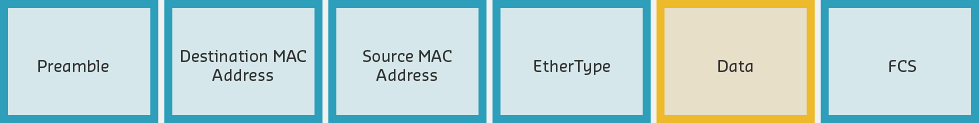
Frame header contains: - Destination MAC address: Where is this frame going? - Source MAC address: Where did this frame come from? - Type/Length: What protocol is in the payload? - Payload: Actual data (IP packet) - Frame Check Sequence: Error detection

652.4.3 MAC Address Format

Figure 652.5: MAC address OUI (Organizationally Unique Identifier) vendor assignment

Structure: 48 bits (6 bytes) = 12 hexadecimal digits

Common formats: - 01-23-45-67-89-AB (hyphens) - 01:23:45:67:89:AB (colons - most common) - 0123.4567.89AB (dots - Cisco style) - 0123456789AB (no separators - printed on labels)

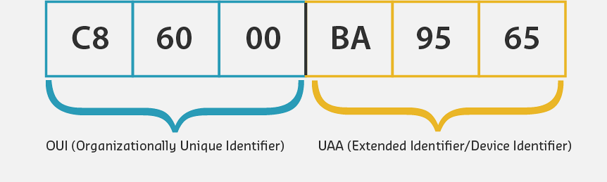
652.4.4 OUI (Organizationally Unique Identifier)

First 24 bits identify the manufacturer:

%% fig-alt: "MAC address OUI structure showing the 48-bit address divided into two parts: the first 24 bits form the Organizationally Unique Identifier (OUI) assigned to the manufacturer, and the remaining 24 bits form the Device ID uniquely assigned by the manufacturer"
%%{init: {'theme': 'base', 'themeVariables': {'primaryColor': '#2C3E50', 'primaryTextColor': '#fff', 'primaryBorderColor': '#16A085', 'lineColor': '#16A085', 'secondaryColor': '#E67E22', 'tertiaryColor': '#7F8C8D'}}}%%
graph LR
    subgraph MAC["MAC Address: 00:1A:2B:3C:4D:5E"]
        subgraph OUI["OUI (First 24 bits)"]
            B1["00"]
            B2["1A"]
            B3["2B"]
        end
        subgraph DevID["Device ID (Last 24 bits)"]
            B4["3C"]
            B5["4D"]
            B6["5E"]
        end
    end

    OUI_Label["Manufacturer<br/>(Assigned by IEEE)"]
    Dev_Label["Unique Device<br/>(Assigned by Vendor)"]

    OUI -.-> OUI_Label
    DevID -.-> Dev_Label

    style B1 fill:#16A085,stroke:#2C3E50,color:#fff
    style B2 fill:#16A085,stroke:#2C3E50,color:#fff
    style B3 fill:#16A085,stroke:#2C3E50,color:#fff
    style B4 fill:#E67E22,stroke:#2C3E50,color:#fff
    style B5 fill:#E67E22,stroke:#2C3E50,color:#fff
    style B6 fill:#E67E22,stroke:#2C3E50,color:#fff
    style OUI_Label fill:#16A085,stroke:#2C3E50,color:#fff
    style Dev_Label fill:#E67E22,stroke:#2C3E50,color:#fff

Figure 652.6: MAC Address OUI structure - First 24 bits identify the manufacturer, last 24 bits are device-specific

Example OUIs: - 00:1A:2B - Cisco Systems - A4:CF:12 - Espressif (ESP32 manufacturer) - B8:27:EB - Raspberry Pi Foundation - DC:A6:32 - Raspberry Pi Trading

Lookup: IEEE OUI Search

652.4.5 Types of MAC Addresses

Type	Address	Purpose	Example
Unicast	Unique device address	One-to-one communication	`A4:CF:12:34:56:78`
Broadcast	All 1s	Send to all devices on network	`FF:FF:FF:FF:FF:FF`
Multicast	Group address	Send to specific group	`01:00:5E:xx:xx:xx`

IoT Note: Wireless MAC addresses may not be constant (privacy features), but each MAC on a network segment must be unique.

Alternative View: MAC vs IP Address Comparison

This variant presents the key differences between Layer 2 (MAC) and Layer 3 (IP) addressing side-by-side:

%%{init: {'theme': 'base', 'themeVariables': { 'primaryColor': '#2C3E50', 'primaryTextColor': '#fff', 'primaryBorderColor': '#16A085', 'lineColor': '#E67E22', 'secondaryColor': '#16A085'}}}%%
graph TB
    subgraph MAC["MAC Address (Layer 2)"]
        M1["48 bits = 6 bytes"]
        M2["Burned into NIC"]
        M3["Flat namespace"]
        M4["Local delivery only"]
        M5["Example: A4:CF:12:34:56:78"]
    end

    subgraph IP["IP Address (Layer 3)"]
        I1["32 bits (IPv4) or 128 bits (IPv6)"]
        I2["Assigned by DHCP or static"]
        I3["Hierarchical (network.host)"]
        I4["Global routing"]
        I5["Example: 192.168.1.100"]
    end

    MAC -->|"Used by"| SW["Switch<br/>Forwards frames"]
    IP -->|"Used by"| RT["Router<br/>Forwards packets"]

    style M1 fill:#16A085,stroke:#2C3E50,color:#fff
    style M2 fill:#16A085,stroke:#2C3E50,color:#fff
    style M3 fill:#16A085,stroke:#2C3E50,color:#fff
    style M4 fill:#16A085,stroke:#2C3E50,color:#fff
    style M5 fill:#16A085,stroke:#2C3E50,color:#fff
    style I1 fill:#E67E22,stroke:#2C3E50,color:#fff
    style I2 fill:#E67E22,stroke:#2C3E50,color:#fff
    style I3 fill:#E67E22,stroke:#2C3E50,color:#fff
    style I4 fill:#E67E22,stroke:#2C3E50,color:#fff
    style I5 fill:#E67E22,stroke:#2C3E50,color:#fff
    style SW fill:#2C3E50,stroke:#16A085,color:#fff
    style RT fill:#2C3E50,stroke:#16A085,color:#fff

MAC addresses work on local network segments (same switch), while IP addresses enable routing across different networks.

Alternative View: Frame vs Packet Encapsulation

This variant shows how IP packets are encapsulated inside Ethernet frames for transmission:

%%{init: {'theme': 'base', 'themeVariables': { 'primaryColor': '#2C3E50', 'primaryTextColor': '#fff', 'primaryBorderColor': '#16A085', 'lineColor': '#E67E22', 'secondaryColor': '#16A085'}}}%%
graph LR
    subgraph FRAME["Ethernet Frame (Layer 2)"]
        FH["Frame Header<br/>Dest MAC, Src MAC"]
        subgraph PACKET["IP Packet (Layer 3)"]
            PH["Packet Header<br/>Dest IP, Src IP"]
            subgraph SEG["TCP/UDP (Layer 4)"]
                SH["Segment<br/>Port numbers"]
                DATA["Application Data"]
            end
        end
        FT["FCS"]
    end

    FH --> PH --> SH --> DATA --> FT

    style FH fill:#2C3E50,stroke:#16A085,color:#fff
    style PH fill:#16A085,stroke:#2C3E50,color:#fff
    style SH fill:#E67E22,stroke:#2C3E50,color:#fff
    style DATA fill:#7F8C8D,stroke:#2C3E50,color:#fff
    style FT fill:#2C3E50,stroke:#16A085,color:#fff

Each layer adds its own header containing addressing information for that layer. This is encapsulation - layers wrap around each other like envelopes.

652.5 Internet Layer: IP Addressing

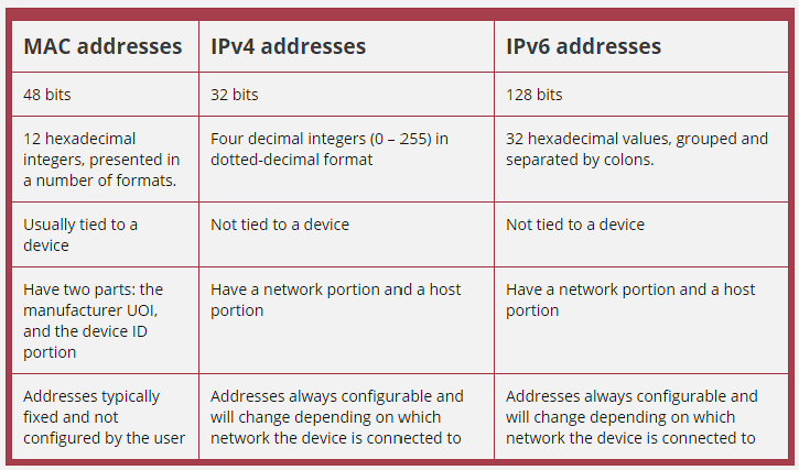
652.5.1 IPv4 vs MAC Addresses

Key difference: MAC addresses are typically fixed (burned into hardware), while IP addresses are configurable and change based on network.

652.5.2 IPv4 Address Structure

Size: 32 bits (4 bytes)

Format: Four octets separated by dots (dotted-decimal notation)

Examples: - 10.0.122.57 - 172.16.11.202 - 192.168.100.4

Conversion: - Each octet: 0-255 (8 bits) - 10.0.122.57 in binary: 00001010.00000000.01111010.00111001

652.6 IPv4 Subnet Masks

Figure 652.9: IPv4 subnet mask examples showing CIDR notation and network division

652.6.1 Purpose

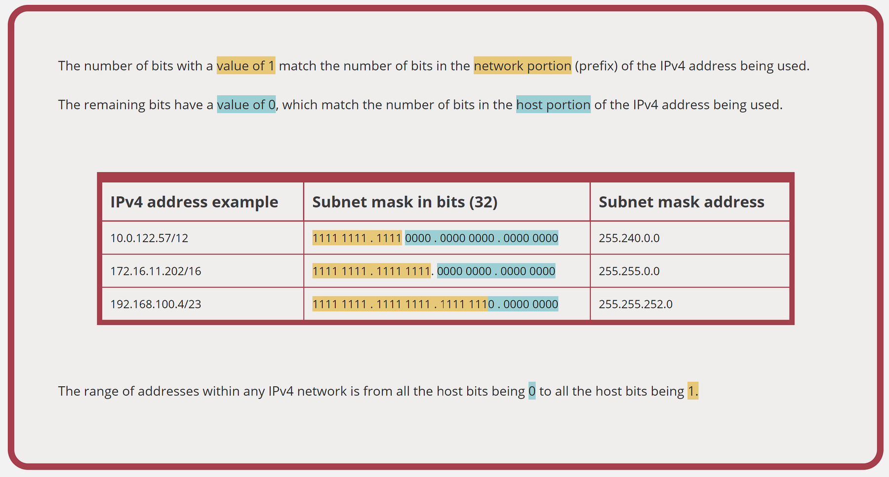
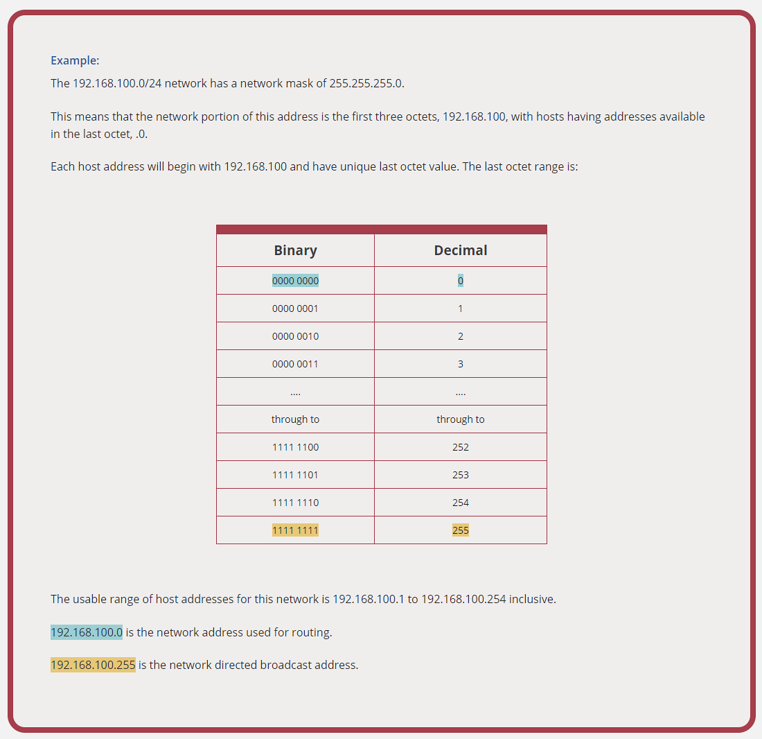
Subnet mask determines which part of the IP address is the network portion and which is the host portion.

652.6.2 Binary Perspective

Subnet mask: Most significant bits are 1, least significant bits are 0

Example:

%% fig-alt: "Subnet mask binary breakdown showing IP address 192.168.1.100 and subnet mask 255.255.255.0 in both decimal and binary format. The binary representation shows how the first 24 bits (all 1s in the mask) identify the network portion, while the last 8 bits (all 0s in the mask) identify the host portion"
%%{init: {'theme': 'base', 'themeVariables': {'primaryColor': '#2C3E50', 'primaryTextColor': '#fff', 'primaryBorderColor': '#16A085', 'lineColor': '#16A085', 'secondaryColor': '#E67E22', 'tertiaryColor': '#7F8C8D'}}}%%
graph TB
    subgraph IP["IP Address: 192.168.1.100"]
        IP1["192<br/>11000000"]
        IP2["168<br/>10101000"]
        IP3["1<br/>00000001"]
        IP4["100<br/>01100100"]
    end

    subgraph Mask["Subnet Mask: 255.255.255.0"]
        M1["255<br/>11111111"]
        M2["255<br/>11111111"]
        M3["255<br/>11111111"]
        M4["0<br/>00000000"]
    end

    subgraph Result["Network/Host Division"]
        Net["Network Portion<br/>192.168.1<br/>(First 24 bits)"]
        Host["Host Portion<br/>.100<br/>(Last 8 bits)"]
    end

    IP1 --> M1
    IP2 --> M2
    IP3 --> M3
    IP4 --> M4

    M1 --> Net
    M2 --> Net
    M3 --> Net
    M4 --> Host

    style IP1 fill:#16A085,stroke:#2C3E50,color:#fff
    style IP2 fill:#16A085,stroke:#2C3E50,color:#fff
    style IP3 fill:#16A085,stroke:#2C3E50,color:#fff
    style IP4 fill:#E67E22,stroke:#2C3E50,color:#fff
    style M1 fill:#16A085,stroke:#2C3E50,color:#fff
    style M2 fill:#16A085,stroke:#2C3E50,color:#fff
    style M3 fill:#16A085,stroke:#2C3E50,color:#fff
    style M4 fill:#E67E22,stroke:#2C3E50,color:#fff
    style Net fill:#16A085,stroke:#2C3E50,color:#fff
    style Host fill:#E67E22,stroke:#2C3E50,color:#fff

Figure 652.11: Subnet mask binary breakdown - showing how mask bits separate network and host portions

Result: - Network: 192.168.1.0 (where all host bits = 0) - Hosts: 192.168.1.1 to 192.168.1.254 - Broadcast: 192.168.1.255 (where all host bits = 1)

652.6.3 Common Subnet Masks

Mask	CIDR	Network Bits	Host Bits	# of Hosts	Use Case
`255.255.255.252`	/30	30	2	2	Point-to-point links
`255.255.255.0`	/24	24	8	254	Small networks
`255.255.0.0`	/16	16	16	65,534	Large networks
`255.0.0.0`	/8	8	24	16,777,214	Huge networks

652.6.4 Calculating Available Hosts

Formula: 2^(host bits) - 2

Why -2? - Network address (all host bits = 0) - used for routing - Broadcast address (all host bits = 1) - used for broadcast

Example: 255.255.255.0 (/24) - Host bits: 8 - Total addresses: 2^8 = 256 - Usable hosts: 256 - 2 = 254

📹 Video: Subnet Mask Explained

Understanding subnet masks: Subnet Mask Explained

Visualizing subnet masks: Visualizing the Subnet Mask

Essential for IP network configuration and troubleshooting.

652.7 IPv6: The Future of IP Addressing

652.7.1 Why IPv6?

The Problem: - IPv4: 32 bits = ~4.3 billion addresses - Problem: IPv4 addresses exhausted! - IoT needs: Trillions of devices - NAT workaround: Complex, breaks end-to-end connectivity

The Solution: - IPv6: 128 bits = 3.4 × 10^38 addresses - Enough to assign: ~670 million addresses per square millimeter of Earth’s surface!

652.7.2 IPv6 Address Structure

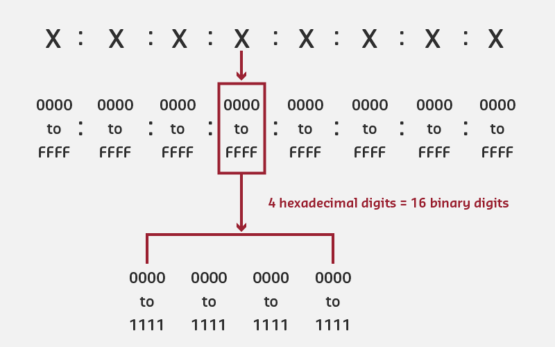
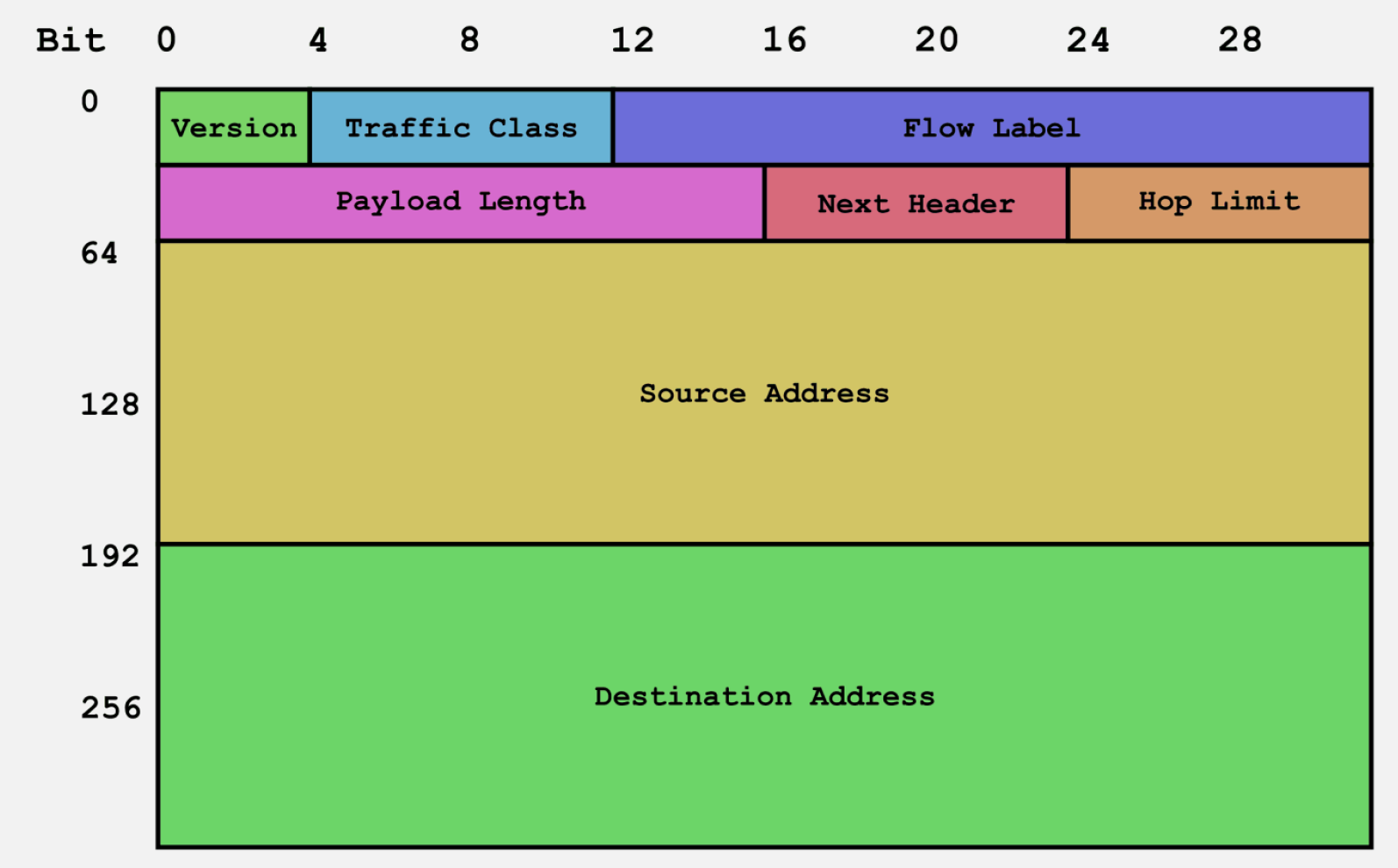
IPv6 header — Figure 652.14: IPv6 packet header format simplified from IPv4 for improved routing efficiency

IPv6 examples — Figure 652.15: Example IPv6 addresses showing different address types and formats

Size: 128 bits (16 bytes)

Format: Eight groups of 16 bits (hextets), separated by colons

Full address example:

2001:0DB8:0000:0000:0000:0000:0000:0001

Representation: Each hextet = 4 hexadecimal digits (0-9, A-F)

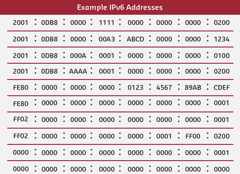
652.7.3 IPv6 Address Compression

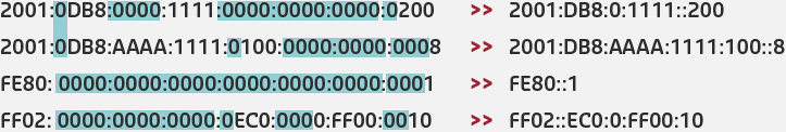
Compressed IPv6 addresses — Figure 652.17: IPv6 address compression rules for shortening address notation

Rules to shorten IPv6 addresses:

Remove leading zeros in each hextet
Replace consecutive groups of zeros with ::

Example compressions:

Original	Compressed	Notes
`2001:0DB8:0000:0000:0000:0000:0000:0001`	`2001:DB8::1`	Removed leading zeros, replaced zeros with `::`
`FE80:0000:0000:0000:0202:B3FF:FE1E:8329`	`FE80::202:B3FF:FE1E:8329`	Replaced middle zeros
`FF02:0000:0000:0000:0000:0000:0000:0001`	`FF02::1`	Multicast all-nodes address
`0000:0000:0000:0000:0000:0000:0000:0001`	`::1`	Localhost (loopback)
`0000:0000:0000:0000:0000:0000:0000:0000`	`::`	Unspecified address

Important: :: can only appear once in an address!

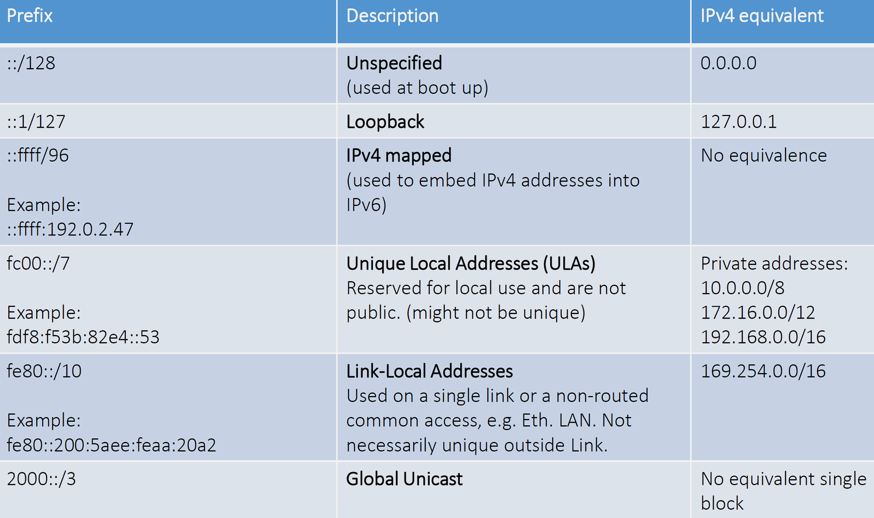
652.7.4 IPv6 Prefix Notation

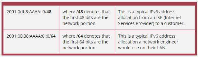
Unicast addresses — Figure 652.19: IPv6 unicast address types - global, link-local, and unique local

No subnet masks needed! IPv6 uses prefix length instead.

Format: address/prefix

Example:

%% fig-alt: "IPv6 prefix notation breakdown showing address 2001:DB8:ACAD:1::1/64 divided into network prefix (first 64 bits: 2001:DB8:ACAD:1) and interface identifier (last 64 bits: ::1). The /64 suffix indicates the prefix length in bits"
%%{init: {'theme': 'base', 'themeVariables': {'primaryColor': '#2C3E50', 'primaryTextColor': '#fff', 'primaryBorderColor': '#16A085', 'lineColor': '#16A085', 'secondaryColor': '#E67E22', 'tertiaryColor': '#7F8C8D'}}}%%
graph TB
    Full["Full Address: 2001:DB8:ACAD:1::1/64"]

    subgraph Prefix["Network Prefix (First 64 bits)"]
        P1["2001"]
        P2["DB8"]
        P3["ACAD"]
        P4["1"]
    end

    subgraph IID["Interface Identifier (Last 64 bits)"]
        I1["0000"]
        I2["0000"]
        I3["0000"]
        I4["0001"]
    end

    Notation["/64 = 64-bit prefix length"]

    Full --> Prefix
    Full --> IID
    Full --> Notation

    style Full fill:#2C3E50,stroke:#16A085,color:#fff
    style P1 fill:#16A085,stroke:#2C3E50,color:#fff
    style P2 fill:#16A085,stroke:#2C3E50,color:#fff
    style P3 fill:#16A085,stroke:#2C3E50,color:#fff
    style P4 fill:#16A085,stroke:#2C3E50,color:#fff
    style I1 fill:#E67E22,stroke:#2C3E50,color:#fff
    style I2 fill:#E67E22,stroke:#2C3E50,color:#fff
    style I3 fill:#E67E22,stroke:#2C3E50,color:#fff
    style I4 fill:#E67E22,stroke:#2C3E50,color:#fff
    style Notation fill:#7F8C8D,stroke:#2C3E50,color:#fff

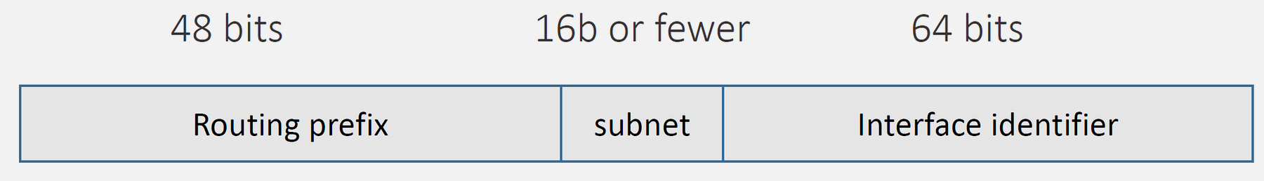
Figure 652.20: IPv6 prefix notation - /64 indicates 64-bit network prefix with 64-bit interface identifier

Network and Host Portions: - Network prefix (first 64 bits): 2001:DB8:ACAD:1 - Interface identifier (last 64 bits): ::1

Standard allocation: - /64 for end networks (LANs) - /48 for sites/organizations - /32 for ISPs

652.7.5 IPv6 Benefits for IoT

Figure 652.21: Modified EUI-64 format for generating IPv6 interface identifiers from MAC addresses

1. Abundant Addresses - Every device gets unique global address - No NAT complications - End-to-end connectivity

2. Simplified Configuration - Stateless Address Autoconfiguration (SLAAC) - Plug-and-play for IoT devices - DHCPv6 optional, not required

3. Improved Security - IPsec built into IPv6 - Better encryption support - Privacy extensions

4. Efficient Routing - Simplified header structure - Faster packet processing - Hierarchical addressing

652.8 MAC vs IP Addresses: Comparison

Figure 652.23: Address types in networking - physical (MAC) and logical (IP) addressing

Feature	MAC Address	IP Address (IPv4/IPv6)
Layer	Data Link (Layer 2)	Network (Layer 3)
Size	48 bits	32 bits (IPv4) / 128 bits (IPv6)
Assigned by	Manufacturer (OUI + unique)	Network administrator or DHCP
Scope	Local network segment	Global (routable across Internet)
Changes?	Usually fixed (hardware)	Changes when connecting to different networks
Format	`00:1A:2B:3C:4D:5E`	`192.168.1.100` or `2001:DB8::1`
Purpose	Local frame delivery	End-to-end routing
Uniqueness	Globally unique (in theory)	Unique within network

Analogy: - MAC address = Your house (fixed location) - IP address = Your mailing address (changes when you move)

652.9 Address Resolution Protocol (ARP)

ARP protocol — Figure 652.24: Address Resolution Protocol (ARP) mapping IP addresses to MAC addresses

652.9.1 The Problem

To send data on a local network: - Know destination IP address (for routing) - Need destination MAC address (for frame delivery)

How to find the MAC address for a given IP address?

652.9.2 ARP Solution

Address Resolution Protocol (ARP) maps IP addresses to MAC addresses.

652.9.3 ARP Process

1. Host A wants to send data to 192.168.1.20 - Checks ARP cache (table of IP→MAC mappings) - If not found, sends ARP request

2. ARP Request (Broadcast) - Destination MAC: FF:FF:FF:FF:FF:FF (broadcast) - Message: “Who has IP 192.168.1.20? Tell 192.168.1.10” - All hosts on network receive request

3. ARP Reply (Unicast) - Host B recognizes its IP address - Sends reply: “192.168.1.20 is at MAC BB:BB:BB” - Reply sent directly to Host A (unicast)

4. Host A updates ARP cache - Stores mapping: 192.168.1.20 → BB:BB:BB - Cache entry expires after timeout (typically 2-20 minutes) - Now can send Ethernet frames to Host B

652.9.4 IPv6 Equivalent: NDP

Neighbor Discovery Protocol (NDP) serves the same purpose for IPv6: - Maps IPv6 addresses to MAC addresses - Uses ICMPv6 messages - More efficient than ARP - Includes additional features (router discovery, address autoconfiguration)

652.10 💻 Hands-On Labs

652.10.1 Lab 1: Explore Network Configuration

Objective: Examine IP, subnet mask, gateway, and MAC addresses on your device.

652.10.1.1 Windows:

ipconfig /all

Look for: - IPv4 Address - Subnet Mask - Default Gateway - Physical Address (MAC) - DNS Servers

652.10.1.2 macOS/Linux:

ifconfig
# OR
ip addr show

652.10.1.3 ESP32 Code:

#include <Wi-Fi.h>

const char* ssid = "YourNetwork";
const char* password = "YourPassword";

void setup() {
  Serial.begin(115200);
  Wi-Fi.begin(ssid, password);

  while (Wi-Fi.status() != WL_CONNECTED) {
    delay(500);
    Serial.print(".");
  }

  Serial.println("\n\n=== Network Configuration ===");
  Serial.print("IP Address: ");
  Serial.println(Wi-Fi.localIP());
  Serial.print("Subnet Mask: ");
  Serial.println(Wi-Fi.subnetMask());
  Serial.print("Gateway: ");
  Serial.println(Wi-Fi.gatewayIP());
  Serial.print("DNS: ");
  Serial.println(Wi-Fi.dnsIP());
  Serial.print("MAC Address: ");
  Serial.println(Wi-Fi.macAddress());
}

void loop() {
  // Nothing
}

652.10.2 Lab 2: View ARP Table

Objective: See IP-to-MAC address mappings on your system.

652.10.2.1 Windows:

arp -a

652.10.2.2 macOS/Linux:

arp -a
# OR
ip neigh show

Expected output:

Internet Address      Physical Address      Type
192.168.1.1          aa-bb-cc-dd-ee-ff    dynamic
192.168.1.20         11-22-33-44-55-66    dynamic

652.10.3 Lab 3: Subnet Calculation Practice

Given: - IP: 192.168.10.50 - Subnet mask: 255.255.255.0

Calculate: 1. Network address? 2. Broadcast address? 3. First usable host? 4. Last usable host? 5. Number of usable hosts?

Show Answers

Network address: 192.168.10.0
Broadcast address: 192.168.10.255
First usable host: 192.168.10.1
Last usable host: 192.168.10.254
Number of usable hosts: 254 (2^8 - 2)

652.11 Knowledge Check

Test your understanding of network layers, protocol encapsulation, and addressing with these questions.

Auto-Gradable Quick Check

Question: In a 48-bit MAC address, which portion identifies the manufacturer (vendor)?

💡 Explanation: B. The Organizationally Unique Identifier (OUI) is the first 24 bits; the remaining bits are assigned by the vendor per device/interface.

Question: What destination MAC address is used for an Ethernet broadcast frame?

💡 Explanation: D. Broadcast targets every station on the local L2 segment.

Question: In IPv4 networks, which protocol resolves an IP address to a MAC address on the local link?

💡 Explanation: A. Address Resolution Protocol (ARP) maps IPv4 addresses to MAC addresses within a broadcast domain.

Question: In an Ethernet II frame, which field indicates what protocol is carried in the payload (e.g., IPv4 vs ARP)?

💡 Explanation: C. The EtherType identifies the payload protocol (e.g., 0x0800 IPv4, 0x0806 ARP, 0x86DD IPv6).

652.12 🎯 Quiz: Test Your Understanding

Python Implementation: Network Layer Tools

Let’s implement comprehensive Python tools for analyzing network layers, protocol encapsulation, and addressing:

652.12.1 Protocol Encapsulation and Layer Simulator

652.12.2 IPv4/IPv6 Address and Subnet Calculator

652.12.3 ARP Table and MAC/IP Mapping Simulator

652.13 Visual Reference Gallery

AI-Generated Figure Variants for Network Addressing and Layering

These AI-generated SVG figures provide alternative visual representations of network addressing and protocol layering concepts. Each figure uses the IEEE color palette for consistency.

Network layering concept diagram showing how each layer provides services to the layer above while using services from the layer below in a hierarchical stack — Layering Concept

IPv4 address structure diagram showing 32-bit address divided into network and host portions with dotted-decimal notation examples — IPv4 Structure

IPv6 address structure diagram showing 128-bit address format with hexadecimal notation, compression rules, and prefix notation for IoT networks — IPv6 Structure

ARP resolution process diagram showing broadcast request for IP-to-MAC mapping, unicast reply, and ARP cache update for local network frame delivery — ARP Process

Protocol encapsulation diagram showing data wrapped with headers at each layer from Application through Physical with PDU names at each level — Encapsulation

652.14 Additional Visual References

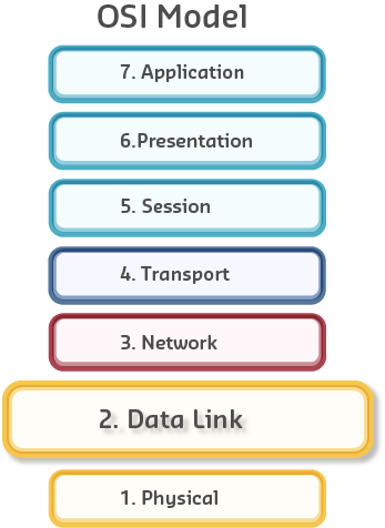
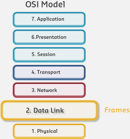
Visual: OSI Model Layers

OSI 7-layer model diagram showing Physical, Data Link, Network, Transport, Session, Presentation, and Application layers with their functions and example protocols at each layer

OSI Model

The OSI model provides the theoretical framework for understanding network communication, with each layer performing specific functions from physical transmission to application services.

Visual: Data Link Layer Functions

Data link layer diagram showing its position between network and physical layers, with responsibilities including framing, MAC addressing, error detection with CRC, and media access control

Data Link Layer

The Data Link layer handles MAC addressing, framing, and error detection - critical functions for local network frame delivery between adjacent devices.

Visual: Encapsulation and Decapsulation

Protocol encapsulation diagram showing how application data is wrapped with headers at each layer creating segments, packets, and frames during transmission, and unwrapped during reception

Encapsulation Process

Understanding encapsulation reveals how data transforms as it passes through network layers, with each layer adding its own header for addressing and control.

652.15 Summary

This chapter provided hands-on implementation of network addressing and protocol layering concepts:

MAC addresses (48-bit) identify network interfaces at Layer 2, with first 24 bits (OUI) identifying manufacturer and last 24 bits providing device-specific identifier
IPv4 addressing (32-bit) uses dotted-decimal notation with subnet masks to divide networks into network and host portions, enabling hierarchical routing
Subnet masks determine network boundaries: /24 provides 254 usable hosts, /30 provides 2 (point-to-point links), calculated as 2^(host bits) - 2 (network + broadcast reserved)
IPv6 (128-bit) solves address exhaustion with 340 undecillion addresses, supporting auto-configuration (SLAAC), built-in security (IPsec), and compression (6LoWPAN) for IoT
ARP (Address Resolution Protocol) maps Layer 3 IP addresses to Layer 2 MAC addresses through broadcast requests and unicast replies, enabling local frame delivery
Encapsulation simulator demonstrates header addition at each layer: application data → UDP/TCP segment → IP packet → Ethernet frame → physical bits
Python implementations provide practical tools: IPv4/IPv6 calculators, subnet planners, ARP table simulators, and protocol overhead analyzers showing efficiency vs payload size

652.16 What’s Next

Having implemented addressing and analyzed protocol encapsulation, consolidate your understanding with comprehensive review and assessment:

Layered Models: Review: Test mastery of OSI/TCP-IP models, encapsulation, addressing, and IoT reference architectures with scenario-based questions
Routing protocols: Explore how routers use routing tables and algorithms to guide packets across networks using the Layer 3 addresses you’ve learned
Wireless IoT technologies: Apply layering concepts to Wi-Fi, Bluetooth LE, LoRaWAN, and Zigbee, understanding which OSI layers each technology implements
Network design patterns: Design complete IoT networks from edge sensors through gateways to cloud, selecting appropriate protocols and addressing schemes at each layer