%%{init: {'theme': 'base', 'themeVariables': { 'primaryColor': '#2C3E50', 'primaryTextColor': '#fff', 'primaryBorderColor': '#16A085', 'lineColor': '#16A085', 'secondaryColor': '#E67E22', 'tertiaryColor': '#ECF0F1', 'fontFamily': 'Inter, system-ui, sans-serif'}}}%%
graph TD
    FLOAT["Floating Point<br/>Algorithm<br/>(Matlab/Python)"] --> DESIGN["Design &<br/>Simulation"]
    DESIGN --> CONVERT["Convert to<br/>Fixed Point<br/>Qn.m Format"]
    CONVERT --> SELECT["Select n and m<br/>based on range"]

    SELECT --> Q54["Example: Q5.4<br/>(9 bits total)"]
    Q54 --> RANGE["n=5 integer bits<br/>(sign + 4 bits)<br/>Range: -16.0 to +15.9375"]
    Q54 --> PRECISION["m=4 fractional bits<br/>Resolution: 1/16 = 0.0625"]

    SELECT --> Q15["Example: Q15<br/>(16 bits total)"]
    Q15 --> RANGE2["n=1 sign bit<br/>m=15 fractional<br/>Range: -1.0 to +0.999"]

    CONVERT --> IMPL["Implement on<br/>Fixed-Point Processor<br/>or ASIC"]

    style FLOAT fill:#E67E22,stroke:#2C3E50,stroke-width:2px,color:#fff
    style CONVERT fill:#3498DB,stroke:#2C3E50,stroke-width:2px,color:#fff
    style Q54 fill:#16A085,stroke:#2C3E50,stroke-width:2px,color:#fff
    style Q15 fill:#16A085,stroke:#2C3E50,stroke-width:2px,color:#fff
    style IMPL fill:#2C3E50,stroke:#16A085,stroke-width:2px,color:#fff
1624 Fixed-Point Arithmetic for Embedded Systems
1624.1 Learning Objectives
By the end of this chapter, you will be able to:
- Understand Qn.m format: Define and work with fixed-point number representations
- Convert floating-point to fixed-point: Transform algorithms from float to efficient integer operations
- Select appropriate n and m values: Choose bit allocation based on range and precision requirements
- Implement fixed-point operations: Perform multiplication, division, and other arithmetic correctly
- Evaluate trade-offs: Compare precision loss against performance and power savings
1624.2 Prerequisites
Before diving into this chapter, you should be familiar with:
- Software Optimization: Understanding compiler optimizations and code efficiency
- Optimization Fundamentals: Understanding why optimization matters for IoT
- Binary number representation: Familiarity with how integers are stored in binary
1624.3 Fixed-Point Arithmetic
1624.3.1 Why Fixed-Point?
- Algorithms developed in floating point (Matlab, Python)
- Floating point processors/hardware are expensive!
- Fixed point processors common in embedded systems
- After design and test, convert to fixed point
- Port onto fixed point processor or ASIC
1624.3.2 Qn.m Format
{fig-alt=“Fixed-point arithmetic workflow showing conversion from floating-point algorithm through Qn.m format selection with examples of Q5.4 (9-bit with range -16 to +15.9375) and Q15 (16-bit with range -1 to +0.999) to implementation on fixed-point processor or ASIC”}
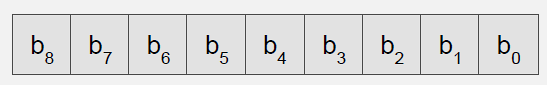
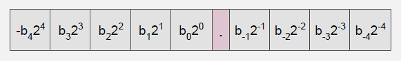
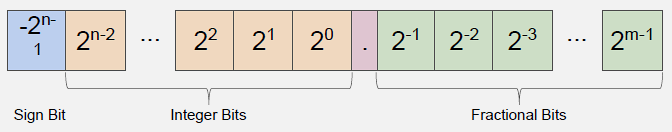
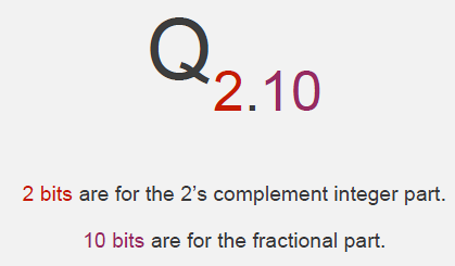
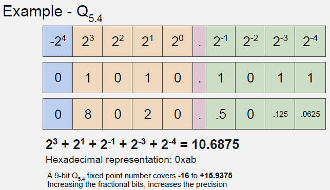
Qn.m Format: Fixed positional number system - n bits to left of decimal (including sign bit) - m bits to right of decimal point - Total bits: n + m
Example - Q5.4 (9 bits total): - 5 bits for integer (sign + 4 bits) - 4 bits for fraction - Range: -16.0 to +15.9375 - Resolution: 1/16 = 0.0625
1624.3.3 Conversion to Qn.m
- Define total number of bits (e.g., 9 bits)
- Fix location of decimal point based on value range
- Determine n and m based on required range and precision
Range Determination: - Run simulations for all input sets - Observe ranges of values for all variables - Note minimum + maximum value each variable sees - Determine Qn.m format to cover range
1624.3.4 Fixed-Point Operations
Addition and Subtraction: Straightforward when formats match
// Q15 + Q15 = Q15 (same format)
int16_t a = 16384;  // 0.5 in Q15
int16_t b = 8192;   // 0.25 in Q15
int16_t c = a + b; // 24576 = 0.75 in Q15Multiplication: Requires renormalization
// Q15 x Q15 = Q30, must shift back to Q15
int16_t a = 16384;  // 0.5 in Q15
int16_t b = 16384;  // 0.5 in Q15
int32_t temp = (int32_t)a * b;  // 268435456 in Q30
int16_t result = temp >> 15; // 8192 = 0.25 in Q15Division: Often avoided or replaced with multiplication by reciprocal
// Divide by 10 using multiply by 0.1 (avoid slow division)
// 0.1 in Q15 = 3277
int16_t x = 32767;  // ~1.0 in Q15
int32_t temp = (int32_t)x * 3277;  // Multiply by 0.1
int16_t result = temp >> 15;        // ~3277 = ~0.1
1624.4 Knowledge Check
TipUnderstanding Check: Fixed-Point vs Floating-Point for Edge ML
Scenario: Your edge AI camera runs object detection (MobileNet) on images. Baseline uses float32 (32-bit floating-point), consuming 150mW during inference and requiring 8 MB RAM (model + activations). Latency: 2 seconds/frame on ARM Cortex-M7 @ 200 MHz. You’re evaluating int8 quantization (8-bit fixed-point), which the datasheet claims provides 4x speedup and 4x memory reduction with <2% accuracy loss.
Think about: 1. What are the new latency, RAM, and power metrics with int8 quantization? 2. Does 4x speedup enable real-time processing (30 fps = 33ms/frame)? 3. What additional considerations affect the decision beyond performance metrics?
Key Insight: Int8 quantization benefits: Latency: 2 sec / 4 = 500ms/frame (still far from 33ms real-time, but 4x better). RAM: 8 MB / 4 = 2 MB (fits in devices with 4 MB SRAM vs requiring 16 MB). Power: ~150mW / 4 = ~38mW (longer battery life or enables smaller battery). Verdict: Use int8 quantization. While 500ms still isn’t real-time, it’s “good enough” for many applications (e.g., doorbell detection every 0.5 sec is fine). The 2 MB RAM savings enables deployment on cheaper hardware ($5 MCU with 4 MB RAM vs $15 MCU with 16 MB RAM). Trade-off: <2% accuracy loss is acceptable for most object detection tasks. Non-performance consideration: Some MCUs have hardware int8 accelerators (e.g., ARM Cortex-M55 with Helium vector extension) providing 10-20x additional speedup, potentially reaching real-time. The chapter’s lesson: “Floating point processors/hardware are expensive! Fixed point processors common in embedded systems” - for edge AI, int8 fixed-point is standard.
1624.5 Common Fixed-Point Formats
| Format | Total Bits | Integer | Fractional | Range | Resolution | Use Case |
|---|---|---|---|---|---|---|
| Q1.7 | 8 | 1 | 7 | -1 to +0.992 | 0.0078 | Audio samples |
| Q1.15 (Q15) | 16 | 1 | 15 | -1 to +0.999 | 0.000031 | DSP, audio |
| Q8.8 | 16 | 8 | 8 | -128 to +127.996 | 0.0039 | Sensor data |
| Q16.16 | 32 | 16 | 16 | -32768 to +32767.999 | 0.000015 | GPS coordinates |
| Q1.31 (Q31) | 32 | 1 | 31 | -1 to +0.9999999995 | 4.7e-10 | High-precision DSP |
1624.6 Implementation Tips
Overflow Handling:
// Saturating addition (prevents wraparound)
int16_t saturate_add(int16_t a, int16_t b) {
    int32_t sum = (int32_t)a + b;
    if (sum > 32767) return 32767;
    if (sum < -32768) return -32768;
    return (int16_t)sum;
}
Lookup Tables: For transcendental functions (sin, cos, log, exp)
// Q15 sine lookup table (256 entries for 0 to 2*pi)
const int16_t sin_table[256] = { 0, 804, 1608, 2410, ... };

int16_t fast_sin_q15(uint8_t angle) {
    return sin_table[angle];
}
Scaling for Mixed Formats:
// Convert Q8.8 to Q1.15 (different scaling)
// Q8.8: 1.0 = 256, Q1.15: 1.0 = 32768
// Scale factor: 32768/256 = 128 = shift left by 7
int16_t q88_to_q15(int16_t q88_value) {
    // First clamp to valid Q15 range (-1 to +1)
    if (q88_value > 255) q88_value = 255;   // >1.0 in Q8.8
    if (q88_value < -256) q88_value = -256; // <-1.0 in Q8.8
    return q88_value << 7;
}
1624.7 Key Concepts Summary
Optimization Layers: - Algorithmic: Algorithm selection and design - Software: Code implementation, compiler flags - Microarchitectural: CPU execution patterns - Hardware: Component selection, specialization - System: Integration of all layers
Profiling and Measurement: - Performance counters: Cycles, cache misses, branch prediction - Memory analysis: Bandwidth, latency, alignment - Power profiling: Per-core, per-component consumption - Bottleneck identification: Critical path analysis - Statistical validation: Representative workloads
Fixed-Point Arithmetic: - Lower area/power than floating-point - Precision trade-off management - Integer operations: Fast and efficient - Common in DSP, vision, ML inference
1624.8 Summary
Fixed-point arithmetic enables efficient computation on resource-constrained IoT devices:
- Qn.m Format: n integer bits + m fractional bits provide predictable range and precision
- Conversion Process: Profile floating-point algorithm, determine value ranges, select format
- Operations: Addition is straightforward; multiplication requires renormalization (right shift)
- Trade-offs: Precision loss vs. 4x+ performance gain and significant power savings
- ML Quantization: int8 quantization is standard for edge AI, providing 4x memory and speed benefits
- Implementation: Use saturating arithmetic, lookup tables, and careful overflow handling
The key insight: floating-point hardware is expensive and power-hungry. For IoT devices, fixed-point arithmetic offers a compelling trade-off of slight precision loss for dramatic efficiency gains.
NoteRelated Chapters & Resources
Design Deep Dives: - Energy Considerations - Power optimization - Hardware Prototyping - Hardware design - Reading Spec Sheets - Component selection
Architecture: - Edge Compute - Edge optimization - WSN Overview - Sensor network design
Sensing: - Sensor Circuits - Circuit optimization
Interactive Tools: - Simulations Hub - Power calculators
Learning Hubs: - Quiz Navigator - Design quizzes
1624.9 What’s Next
Having covered optimization fundamentals, hardware strategies, software techniques, and fixed-point arithmetic, you’re now equipped to make informed optimization decisions for IoT systems. The next section covers Reading a Spec Sheet, which develops skills for interpreting device datasheets and technical specifications to ensure correct hardware selection and integration.