%% fig-alt: "WSN architecture showing sensor nodes (temperature and humidity) sending data through relay nodes via multi-hop routing to a gateway, which connects to cloud for analysis"
%%{init: {'theme': 'base', 'themeVariables': { 'primaryColor': '#2C3E50', 'primaryTextColor': '#fff', 'primaryBorderColor': '#16A085', 'lineColor': '#16A085', 'secondaryColor': '#E67E22', 'tertiaryColor': '#7F8C8D', 'fontSize': '16px'}}}%%
graph TB
    S1[Sensor Node 1<br/>Temp: 22°C] --> R1[Relay Node]
    S2[Sensor Node 2<br/>Temp: 23°C] --> R1
    S3[Sensor Node 3<br/>Humidity: 65%] --> R2[Relay Node]
    S4[Sensor Node 4<br/>Humidity: 68%] --> R2

    R1 -->|Multi-hop| GW[Gateway/<br/>Base Station]
    R2 -->|Multi-hop| GW

    GW -->|Internet| Cloud[Cloud<br/>Analysis]

    style S1 fill:#2C3E50,stroke:#16A085,color:#fff
    style S2 fill:#2C3E50,stroke:#16A085,color:#fff
    style S3 fill:#2C3E50,stroke:#16A085,color:#fff
    style S4 fill:#2C3E50,stroke:#16A085,color:#fff
    style R1 fill:#16A085,stroke:#2C3E50,color:#fff
    style R2 fill:#16A085,stroke:#2C3E50,color:#fff
    style GW fill:#E67E22,stroke:#16A085,color:#fff
    style Cloud fill:#2C3E50,stroke:#16A085,color:#fff
368 WSN Architecture and Applications
368.1 Learning Objectives
By the end of this chapter, you will be able to:
- Explain the three-tier WSN architecture: Understand how sensor nodes, gateways, and backend systems work together
- Trace historical evolution: Describe WSN development from military origins to modern IoT integration
- Identify core characteristics: Explain distributed sensing, self-organization, and resource constraints
- Describe application domains: Apply WSN knowledge to environmental, industrial, agricultural, and smart city scenarios
- Compare network topologies: Analyze trade-offs between star, mesh, and cluster configurations
368.2 🌱 Getting Started (For Beginners)
TipWhat is a Wireless Sensor Network? (Simple Explanation)
Analogy: A WSN is like a team of scouts spread across a forest, each reporting back what they observe. Instead of one person trying to watch everything, many scouts share the job and relay messages to headquarters.
In everyday terms: - 📡 Sensor Node = A small scout with a radio and battery - 🏠 Base Station/Gateway = Headquarters that collects all reports - 🔗 Multi-hop = Scouts passing messages through each other (like a relay race)
368.2.1 How WSNs Work (Visual Overview)
Many cheap sensors working together outperform one expensive sensor
368.2.2 Real-World Examples
| Application | What Sensors Measure | Why WSN? |
|---|---|---|
| Smart Farm | Soil moisture, temperature | Fields are huge; one sensor can’t cover everything |
| Forest Fire Detection | Smoke, temperature | Fires can start anywhere; need eyes everywhere |
| Bridge Monitoring | Vibration, stress | Bridges are long; sensors at each point detect problems |
| Wildlife Tracking | Animal location, movement | Animals roam; sensors track migration patterns |
368.2.3 The Key Challenge: Battery Life
%% fig-alt: "Pie chart showing sensor node energy consumption breakdown: Radio TX/RX 70%, Microcontroller 15%, Sensing 10%, Sleep/Idle 5%"
%%{init: {'theme': 'base', 'themeVariables': { 'primaryColor': '#2C3E50', 'primaryTextColor': '#fff', 'primaryBorderColor': '#16A085', 'lineColor': '#16A085', 'secondaryColor': '#E67E22', 'tertiaryColor': '#7F8C8D', 'fontSize': '16px'}}}%%
%%{init: {'theme':'base', 'themeVariables': {'pieOuterStrokeWidth': '3px'}}}%%
pie title "Sensor Node Energy Consumption"
    "Radio TX/RX" : 70
    "Microcontroller" : 15
    "Sensing" : 10
    "Sleep/Idle" : 5
Alternative View:
%% fig-alt: "Decision tree for reducing WSN energy consumption starting from 70% radio energy, showing three main strategies: reduce transmissions via data aggregation (combine 10 readings into 1, 90% reduction), reduce transmission distance via multi-hop routing (10m hops instead of 100m, 100x power savings using inverse square law), and reduce active time via duty cycling (1% duty cycle gives 100x battery life)"
%%{init: {'theme': 'base', 'themeVariables': {'primaryColor': '#2C3E50', 'primaryTextColor': '#fff', 'primaryBorderColor': '#16A085', 'lineColor': '#16A085', 'secondaryColor': '#E67E22', 'tertiaryColor': '#7F8C8D', 'fontSize': '11px'}}}%%
flowchart TD
    START([Radio TX/RX = 70%<br/>of energy budget])

    S1["Strategy 1:<br/>REDUCE TRANSMISSIONS"]
    S2["Strategy 2:<br/>REDUCE DISTANCE"]
    S3["Strategy 3:<br/>REDUCE ACTIVE TIME"]

    T1["Data Aggregation<br/>Combine 10 readings → 1 packet<br/>Result: 90% fewer TX"]
    T2["Multi-hop Routing<br/>10m hops vs 100m direct<br/>Result: 100× power savings<br/>(inverse square law)"]
    T3["Duty Cycling<br/>Sleep 99% of time<br/>Result: 100× battery life"]

    RESULT([Combined: Transform<br/>4-day battery → 2+ years])

    START --> S1 & S2 & S3
    S1 --> T1
    S2 --> T2
    S3 --> T3
    T1 & T2 & T3 --> RESULT

    style START fill:#E67E22,stroke:#2C3E50,color:#fff
    style S1 fill:#16A085,stroke:#2C3E50,color:#fff
    style S2 fill:#16A085,stroke:#2C3E50,color:#fff
    style S3 fill:#16A085,stroke:#2C3E50,color:#fff
    style T1 fill:#2C3E50,stroke:#16A085,color:#fff
    style T2 fill:#2C3E50,stroke:#16A085,color:#fff
    style T3 fill:#2C3E50,stroke:#16A085,color:#fff
    style RESULT fill:#16A085,stroke:#2C3E50,color:#fff
Radio transmission dominates WSN energy consumption - every design decision should minimize transmissions!
368.2.4 Quick Self-Check
Before continuing, make sure you understand:
- What is a sensor node? → A small device that senses, processes, and wirelessly transmits data
- Why many sensors instead of one? → Coverage, redundancy, and lower cost per area
- What’s the biggest design constraint? → Battery life (energy efficiency)
- What is multi-hop? → Data passing through intermediate nodes to reach the gateway
CautionCommon Misconception: “More Sensors = Better Coverage Always”
The Myth: Deploying more sensor nodes always improves coverage and network reliability.
The Reality: Over-provisioning sensors creates diminishing returns and introduces new problems:
- Energy Hotspots: Dense deployments create contention for the wireless channel, forcing nodes near the sink to relay massive amounts of traffic, depleting their batteries 10-100× faster than edge nodes
- Interference and Collisions: Too many sensors in close proximity increase radio interference, packet collisions, and retransmissions, actually decreasing reliability and throughput
- Cost-Benefit Break Point: Beyond optimal density (typically 5-10 neighbors per node), additional sensors provide minimal coverage improvement but linearly increase hardware, deployment, and maintenance costs
- Calibration Drift: More sensors mean more calibration maintenance—uncalibrated sensors provide redundant but inaccurate data, reducing fusion quality
Better Approach: Use k-coverage analysis (see WSN Coverage Fundamentals) to mathematically determine minimum node density for required coverage level. Deploy redundancy strategically only in critical areas (perimeters, near sinks) rather than uniformly. Consider hybrid topologies: sparse sensing layer + mobile data collectors, or hierarchical clustering with non-uniform node distribution matching application requirements.
Example: A precision agriculture deployment reduced nodes from 500 to 180 using coverage optimization, cutting costs 64% while maintaining 95% area coverage with k=2 redundancy.
369 Wireless Sensor Networks
NoteKey Concepts
- Wireless Sensor Network (WSN): Network of spatially distributed autonomous sensor nodes cooperatively monitoring environmental or physical conditions
- Sensor Node: Small, battery-powered device with sensing, processing, and wireless communication capabilities deployed in monitored environments
- Network Topology: Organization of sensor nodes (star, mesh, cluster, hybrid) affecting communication patterns and energy efficiency
- Data Aggregation: Combining data from multiple sensors to reduce transmission overhead and extract higher-level information
- Energy Efficiency: Primary design constraint for WSNs, dictating node lifetime and determining feasible network operations
- Multi-Hop Communication: Nodes relay data through intermediaries to reach base stations beyond direct radio range
369.1 Overview
Wireless Sensor Networks (WSNs) represent a foundational technology in the Internet of Things ecosystem, consisting of spatially distributed autonomous sensors that cooperatively monitor physical or environmental conditions. These networks have evolved from specialized military and industrial applications to become integral components of modern IoT systems, enabling pervasive sensing across diverse application domains.
TipDefinition
A Wireless Sensor Network (WSN) is a collection of spatially distributed, autonomous sensor nodes that communicate wirelessly to collectively monitor physical or environmental conditions such as temperature, pressure, humidity, motion, vibration, pollutants, or other parameters of interest.
369.1.1 Historical Evolution
Early Development (1980s-1990s): WSNs emerged from military applications, particularly the Distributed Sensor Networks (DSN) program initiated by DARPA. Early systems were expensive, power-hungry, and limited in capability.
Technological Advancement (2000s): Miniaturization of electronics, advances in wireless communication, and improvements in energy efficiency enabled widespread commercial adoption. The Berkeley Mote platform became a landmark development in WSN research.
IoT Integration (2010s-Present): WSNs have become integral to IoT architectures, with standardized protocols (IEEE 802.15.4, Zigbee, LoRaWAN), cloud integration, and edge computing capabilities transforming their role from isolated systems to connected components of larger ecosystems.
NoteHistorical Context: How Wireless Sensor Networks Evolved
Military Origins (1980s): The concept of distributed sensing emerged from DARPA’s Distributed Sensor Networks (DSN) program, which explored networks of acoustic sensors for tracking submarines and ground vehicles. Early nodes cost $10,000+ each, were the size of shoeboxes, and required wired power. The key insight was that many cheap, imperfect sensors could outperform a few expensive, precise ones through collaborative processing.
Smart Dust Vision (1997-2002): UC Berkeley’s Smart Dust project, led by Kris Pister, envisioned millimeter-scale sensors that would “float in the air like dust.” While the mm-scale goal remained aspirational, this project spawned the Berkeley Motes platform and TinyOS operating system that dominated WSN research for a decade. The original Mica motes cost ~$100 each—still expensive, but revolutionary for research.
Landmark Deployments (2002-2005):
- Great Duck Island (2002): 32 Mica motes monitored seabird nesting burrows on a Maine island—one of the first real-world, long-duration WSN deployments. Revealed practical challenges: node failures, clock drift, and the “energy hole” problem near gateways.
- Redwoods Study (2005): 70 nodes placed in 70-meter-tall redwood trees captured unprecedented microclimate data, demonstrating WSN value for environmental science.
- Golden Gate Bridge (2006): 64 accelerometers monitored structural vibrations, pioneering infrastructure monitoring applications.
Protocol Innovation Era (2000-2010): Academic researchers addressed unique WSN constraints with specialized protocols:
- Directed Diffusion (2000): Data-centric routing where queries propagated through the network and data flowed back along established gradients—fundamentally different from address-based Internet routing.
- LEACH (2000): Hierarchical clustering with rotating cluster heads, pioneering energy-balanced data aggregation.
- S-MAC (2002): Sensor-MAC introduced synchronized sleep schedules, trading latency for 10× energy savings over always-on approaches.
- TAG/TinyDB (2003): Treating the sensor network as a queryable database, enabling SQL-like queries over distributed sensors.
Standardization Wave (2003-2015): Research innovations became industry standards:
| Standard | Year | Origin | WSN Contribution |
|---|---|---|---|
| IEEE 802.15.4 | 2003 | Zigbee Alliance + IEEE | Low-power PHY/MAC from WSN research |
| Zigbee | 2004 | Zigbee Alliance | Mesh networking, application profiles |
| 6LoWPAN | 2007 | IETF | IPv6 header compression for constrained nodes |
| RPL | 2012 | IETF | Distance-vector routing for lossy networks |
| LoRaWAN | 2015 | LoRa Alliance | Long-range from spread-spectrum research |
IoT Convergence (2015-Present): The distinction between “WSN” and “IoT” blurred as:
- Commercial platforms (AWS IoT, Azure IoT) absorbed WSN concepts
- Edge computing brought intelligence back to sensor nodes (echoing early WSN processing)
- Machine learning enabled advanced in-network analytics
- Thread and Matter standards unified home/industrial sensing
Key Research Projects and Their Legacy:
| Project | Institution | Year | Lasting Impact |
|---|---|---|---|
| Smart Dust | UC Berkeley | 1997 | Motes platform, TinyOS, WSN community |
| SensorWeb | NASA/JPL | 2000 | Earth observation, autonomous tasking |
| Habitat Monitoring | Intel/Berkeley | 2002 | Practical deployment lessons |
| VigilNet | UVA | 2004 | Military surveillance, target tracking |
| CitySense | Harvard | 2008 | Urban monitoring, participatory sensing |
| WisePlatform | ETH Zurich | 2010 | Reliable industrial WSN |
Why This Matters for Modern IoT:
Protocol Design Decisions: Why does 802.15.4 use 250 kbps? Why does Zigbee limit payloads to 127 bytes? These choices reflect WSN energy constraints, not arbitrary decisions.
Architectural Patterns: Data aggregation, duty cycling, hierarchical clustering, and gradient-based routing—all IoT patterns originated in WSN research.
Energy-First Thinking: The obsession with energy efficiency in IoT protocols stems from WSN deployments where battery replacement was physically impossible.
Research Community: Most IoT researchers trained on WSN problems; SenSys, IPSN, and MobiCom conferences birthed the field.
The Evolution in Numbers:
| Metric | 1999 (Mica1) | 2005 (Mica2) | 2010 (TelosB) | 2020 (Commercial IoT) |
|---|---|---|---|---|
| Node Cost | ~$100 | ~$50 | ~$30 | ~$5-15 |
| Radio Power (TX) | 27 mA | 17 mA | 17 mA | 5-10 mA |
| MCU | 4 MHz | 8 MHz | 8 MHz | 80-240 MHz |
| RAM | 4 KB | 4 KB | 10 KB | 256+ KB |
| Battery Life (typical) | Days | Weeks | Months | Years |
Understanding this evolution explains why modern IoT standards look the way they do—they carry the DNA of two decades of WSN research embedded in every protocol choice and architectural pattern.
369.1.2 Core Characteristics
Distributed Sensing: Multiple sensor nodes deployed across an area provide redundancy, increased coverage, and improved accuracy through collaborative sensing and data fusion.
Wireless Communication: Nodes communicate without physical wiring, enabling deployment in challenging environments and reducing installation costs.
Self-Organization: Networks autonomously configure themselves, adapt to node failures, and optimize routing without centralized coordination.
Resource Constraints: Nodes typically operate under severe constraints in energy, computation, memory, and communication bandwidth.
Application-Specific Design: WSNs are often designed and optimized for specific applications, with hardware and protocols tailored to particular sensing requirements and environmental conditions.
369.1.3 WSN Architecture
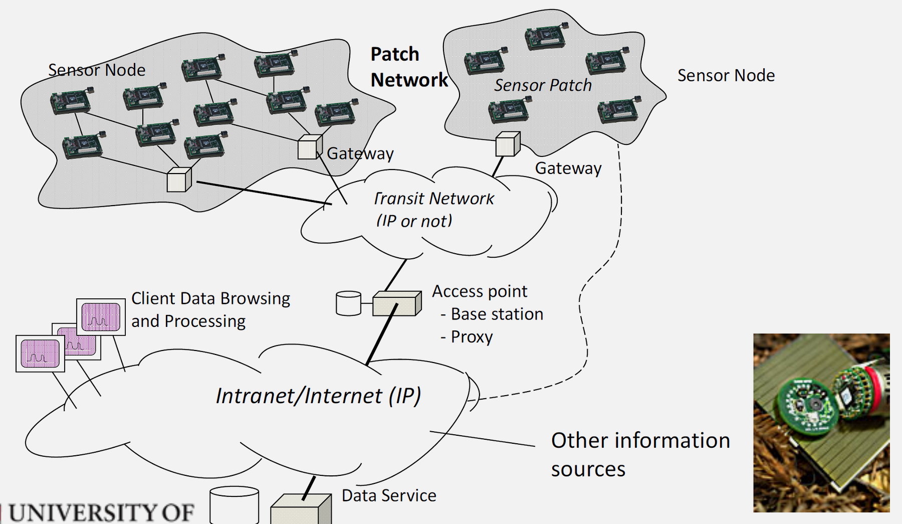
Three-Tier Architecture:
Tier 1 - Sensor Nodes: - Collect environmental data through sensors - Perform local processing and filtering - Transmit data to nearby nodes or gateways - Often battery-powered with limited resources
Tier 2 - Gateway/Sink Nodes: - Aggregate data from multiple sensor nodes - Provide protocol translation (e.g., 802.15.4 to Wi-Fi/Ethernet) - Perform edge processing and data fusion - Connect sensor network to external networks
Tier 3 - Backend Systems: - Cloud or on-premise servers - Store and analyze large-scale data - Provide user interfaces and applications - Enable remote management and configuration
369.1.4 Application Domains
Environmental Monitoring: - Climate and weather monitoring - Pollution detection (air, water, soil) - Forest fire detection - Flood and landslide warning systems - Wildlife habitat monitoring
Industrial Applications: - Structural health monitoring (bridges, buildings, dams) - Machine condition monitoring - Supply chain and inventory tracking - Quality control and process optimization - Hazardous gas detection in industrial facilities
Smart Agriculture: - Precision irrigation management - Soil moisture and nutrient monitoring - Crop health assessment - Livestock tracking and health monitoring - Greenhouse climate control
Healthcare: - Patient vital signs monitoring - Fall detection for elderly care - Hospital asset tracking - Environmental monitoring in medical facilities - Pandemic and disease outbreak detection
Smart Cities: - Traffic monitoring and management - Smart parking systems - Waste management optimization - Street lighting control - Noise level monitoring
Military and Defense: - Battlefield surveillance - Intrusion detection - Target tracking - Chemical/biological threat detection - Equipment and personnel monitoring
369.1.5 Network Topology Visualization
Understanding how sensor nodes organize themselves into network structures is essential for designing effective WSN deployments. The following visualization illustrates common WSN topology patterns.

369.1.6 Cluster-Based Organization
Clustering is a fundamental organization strategy in WSNs where nodes are grouped into clusters, each with a designated cluster head that aggregates data and communicates with the base station.

The clustering approach offers several advantages:
| Benefit | Description |
|---|---|
| Energy Efficiency | Only cluster heads transmit long distances, saving energy for member nodes |
| Scalability | Adding new nodes only requires joining a local cluster |
| Data Aggregation | Cluster heads can combine readings before transmission, reducing traffic |
| Load Balancing | Rotating cluster head role distributes energy consumption |
WarningTradeoff: Star Topology vs Mesh Topology
Option A (Star Topology): All sensor nodes communicate directly with a central gateway/sink. Single-hop communication: 10-50ms latency, no routing overhead. Gateway handles all traffic aggregation. Radio range requirement: nodes must be within 50-100m of gateway. Failure mode: gateway failure = total network failure. Typical deployment: 10-30 nodes in small area (single room, small greenhouse).
Option B (Mesh Topology): Nodes form multi-hop network, forwarding data through neighbors to reach sink. Multi-hop paths: 3-10 hops typical, 100-500ms latency. Distributed routing: each node maintains neighbor table (50-200 bytes). Coverage area: extends to 500m+ through relaying. Failure tolerance: alternate paths available if nodes fail. Typical deployment: 50-1000+ nodes across large areas (farms, forests, cities).
Decision Factors:
- Choose Star Topology when: Coverage area is small (<100m diameter), all nodes within direct range of gateway, latency requirements are strict (<50ms), network size is limited (<30 nodes), or cost/complexity must be minimized (no routing protocol needed).
- Choose Mesh Topology when: Coverage area exceeds single-hop range (>100m), nodes are distributed across irregular terrain or obstacles, fault tolerance is critical (no single point of failure acceptable), or network must scale beyond 50 nodes.
- Quantified comparison: 100-node environmental monitoring. Star (requires 4 gateways for coverage): 100 direct transmissions, 4 gateway installations at $500 each = $2000 infrastructure. Mesh (1 gateway): 100 transmissions + 300 relay transmissions = 400 total, but only $500 infrastructure. Star: lower energy, higher infrastructure cost. Mesh: higher energy, lower infrastructure cost.
WarningTradeoff: Fixed Cluster Head vs Rotating Cluster Head
Option A (Fixed Cluster Head Selection): Cluster heads are predetermined based on node capability (battery size, processing power, location). CHs remain fixed for network lifetime or until failure. Energy consumption: CHs deplete 5-10x faster than members. Typical CH lifetime: 3-6 months with 2000mAh battery. Advantage: stable routing, no CH election overhead (saves 5-10% energy per round). Disadvantage: CHs become network bottleneck and early failure points.
Option B (Rotating Cluster Head Selection): CH role rotates among nodes based on probability and residual energy (LEACH-style). Election overhead: 2-5% additional transmissions per round. Energy distribution: all nodes deplete at similar rate. Network lifetime extended by 40-60% compared to fixed CH. Typical rotation period: every 10-60 minutes. Disadvantage: routing instability during transitions (50-200ms convergence).
Decision Factors:
- Choose Fixed CH when: Some nodes have significantly more resources (mains-powered, larger batteries, better position), network lifetime is short-term (<6 months), routing stability is critical (real-time control applications), or CH election overhead is unacceptable (very low duty cycle networks).
- Choose Rotating CH when: All nodes have similar capabilities (homogeneous network), long network lifetime required (>1 year), energy fairness is important (all nodes should last equally), or network must survive multiple node failures without infrastructure changes.
- Quantified comparison: 200-node network, 2-year target lifetime. Fixed CH (20 CHs, 180 members): CHs fail at 4 months (20× relay traffic), network collapses. Rotating CH (LEACH with p=0.1): all nodes at 15% residual energy at 2 years. Rotating CH achieves 6× longer network operational lifetime.
369.1.7 Sensor Node Hardware Architecture
Understanding the hardware components of sensor nodes helps in designing energy-efficient systems and selecting appropriate platforms for specific applications.


369.2 Summary
This chapter covered the fundamentals of WSN architecture and applications:
- Three-Tier Architecture: Sensor nodes → Gateway/Sink → Backend systems provide hierarchical data flow from distributed sensing to centralized analysis
- Historical Evolution: From DARPA military research (1980s) through Smart Dust vision (1997) to modern IoT integration (2015+)
- Core Characteristics: Distributed sensing, wireless communication, self-organization, resource constraints, and application-specific design
- Application Domains: Environmental monitoring, industrial applications, smart agriculture, healthcare, smart cities, and military/defense
- Network Topologies: Star (simple, limited range), mesh (scalable, fault-tolerant), and cluster (energy-efficient, hierarchical) with trade-offs in energy, complexity, and reliability
369.3 What’s Next
Continue to Sensor Node Characteristics to explore the hardware components, capabilities, and resource constraints of sensor nodes, including multi-hop communication and the critical radio power law that drives WSN protocol design.