%% fig-cap: "GPS Error Budget Breakdown by Source"
%% fig-alt: "Pie chart showing relative contribution of GPS error sources"

%%{init: {'theme': 'base', 'themeVariables': { 'primaryColor': '#2C3E50', 'primaryTextColor': '#fff', 'primaryBorderColor': '#16A085', 'lineColor': '#16A085', 'secondaryColor': '#E67E22', 'tertiaryColor': '#ecf0f1'}}}%%

pie title GPS Error Budget Breakdown
    "Ionospheric Delay (5.0m)" : 5.0
    "Ephemeris Error (2.5m)" : 2.5
    "Satellite Clock (1.5m)" : 1.5
    "Multipath (1.0m)" : 1.0
    "Tropospheric Delay (0.5m)" : 0.5
    "Receiver Noise (0.3m)" : 0.3
1503 GPS Accuracy and Enhancement
1503.1 Learning Objectives
By the end of this chapter, you will be able to:
- Analyze GPS Error Budget: Understand the contribution of each error source to total positioning uncertainty
- Calculate UERE: Apply root-sum-square to combine independent error sources
- Compare Enhancement Technologies: Evaluate DGPS, SBAS, RTK, and PPP for accuracy requirements
- Design for Accuracy Requirements: Select appropriate positioning technology for specific IoT applications
1503.2 Prerequisites
- GPS and Outdoor Positioning: Understanding of GPS fundamentals and error sources
1503.3 GPS Error Budget: Understanding Location Accuracy
Understanding where GPS accuracy comes from—and where it breaks down—is critical for designing reliable IoT location services. A GPS error budget quantifies each error source’s contribution to total positioning uncertainty.
1503.3.1 Error Budget Breakdown
The table below shows the six main error sources, their typical magnitude, how variable they are, and how we can mitigate them:
| Error Source | Typical Error | Notes |
|---|---|---|
| Satellite clock | 1.5 m | Atomic clock drift compensated by ground uploads every 15 minutes |
| Ephemeris data | 2.5 m | Orbital prediction errors; frequent updates every 2 hours minimize drift |
| Ionospheric delay | 5.0 m | Varies with solar activity; equatorial regions 2-3× worse than poles |
| Tropospheric delay | 0.5 m | Weather dependent; humidity and temperature affect signal propagation |
| Multipath | 1.0 m | Urban canyons worst case; signals bounce off buildings creating echoes |
| Receiver noise | 0.3 m | Hardware quality dependent; better RF front-ends reduce noise floor |
| Total (UERE) | ~6 m | Root sum square of all independent error sources |
| With DGPS | <1 m | Differential correction removes common-mode errors (ionosphere, clock) |
| With RTK | <2 cm | Real-time kinematic uses carrier phase for centimeter-level precision |
NoteUnderstanding Error Accumulation
GPS errors don’t simply add up—they combine using root sum square (RSS) because they’re independent random variables:
\[ \text{UERE} = \sqrt{1.5^2 + 2.5^2 + 5.0^2 + 0.5^2 + 1.0^2 + 0.3^2} \approx 6 \text{ meters} \]
Why RSS and not simple addition? If errors added linearly, total would be 10.8 meters. But some errors cancel each other out randomly, resulting in the more realistic 6-meter UERE.
%% fig-cap: "GPS Error Sources Flow: From Satellite to Position Calculation"
%% fig-alt: "Flowchart showing how GPS errors propagate from satellite to receiver"

%%{init: {'theme': 'base', 'themeVariables': { 'primaryColor': '#2C3E50', 'primaryTextColor': '#fff', 'primaryBorderColor': '#16A085', 'lineColor': '#16A085', 'secondaryColor': '#E67E22', 'tertiaryColor': '#ecf0f1', 'noteTextColor': '#2C3E50', 'noteBkgColor': '#fff3cd', 'textColor': '#2C3E50', 'fontSize': '16px'}}}%%

graph TB
    subgraph Satellite["Satellite Segment"]
        SatClock[Satellite Clock<br/>±1.5 m<br/>Atomic clock drift]
        Ephemeris[Ephemeris Error<br/>±2.5 m<br/>Orbital predictions]
    end

    subgraph Atmosphere["Signal Propagation"]
        Iono[Ionospheric Delay<br/>±5.0 m<br/>Charged particles<br/>LARGEST ERROR]
        Tropo[Tropospheric Delay<br/>±0.5 m<br/>Weather effects]
    end

    subgraph Receiver["Receiver Segment"]
        Multi[Multipath<br/>±1.0 m<br/>Urban reflections]
        Noise[Receiver Noise<br/>±0.3 m<br/>Hardware quality]
    end

    subgraph Calculation["Error Combination"]
        RSS[Root Sum Square<br/>UERE = √Σ errors²<br/>≈ 6 meters]
        GDOP[× GDOP Multiplier<br/>Satellite geometry<br/>1.5× to 8.0×]
        Final[Final Position Error<br/>Good: 9m<br/>Poor: 18m<br/>Urban: 48m]
    end

    SatClock --> RSS
    Ephemeris --> RSS
    Iono --> RSS
    Tropo --> RSS
    Multi --> RSS
    Noise --> RSS

    RSS --> GDOP
    GDOP --> Final

    style Iono fill:#E67E22,stroke:#2C3E50,stroke-width:3px,color:#fff
    style RSS fill:#2C3E50,stroke:#16A085,stroke-width:3px,color:#fff
    style Final fill:#16A085,stroke:#2C3E50,stroke-width:3px,color:#fff
    style SatClock fill:#2C3E50,stroke:#16A085,stroke-width:2px,color:#fff
    style Ephemeris fill:#2C3E50,stroke:#16A085,stroke-width:2px,color:#fff
    style Tropo fill:#16A085,stroke:#2C3E50,stroke-width:2px,color:#fff
    style Multi fill:#E67E22,stroke:#16A085,stroke-width:2px,color:#fff
    style Noise fill:#16A085,stroke:#2C3E50,stroke-width:2px,color:#fff
    style GDOP fill:#E67E22,stroke:#16A085,stroke-width:2px,color:#fff
NoteWhy Ionospheric Delay Dominates (45% of Error Budget)
The ionosphere (50-1000 km altitude) is a layer of charged particles created by solar radiation. GPS signals travel through it, and the charged particles slow down the radio waves, making distances appear longer.
Why it’s variable: - Solar activity: During solar storms, ionospheric delay can spike to 10-15 meters (vs. 5m typical) - Time of day: Peak ionization occurs at noon (sun overhead), minimum at night - Geographic location: Equatorial regions have 2-3× higher ionospheric activity than poles
Mitigation: - Dual-frequency receivers: Military (L1 + L2) and modern smartphones (L1 + L5) measure two frequencies and calculate ionospheric delay directly - SBAS augmentation: WAAS (North America), EGNOS (Europe) broadcast ionospheric models - Single-frequency compromise: Civilian L1-only receivers use Klobuchar model (removes ~50% of error)
1503.3.2 Calculating Total GPS Uncertainty (UERE)
UERE (User Equivalent Range Error) is the root-sum-square (RSS) of all error sources, assuming they’re independent and random:
\[ \text{UERE} = \sqrt{\sigma_{\text{clock}}^2 + \sigma_{\text{eph}}^2 + \sigma_{\text{iono}}^2 + \sigma_{\text{tropo}}^2 + \sigma_{\text{multipath}}^2 + \sigma_{\text{noise}}^2} \]
Plugging in typical values:
\[ \text{UERE} = \sqrt{1.5^2 + 2.5^2 + 5.0^2 + 0.5^2 + 1.0^2 + 0.3^2} = \sqrt{2.25 + 6.25 + 25.0 + 0.25 + 1.0 + 0.09} \]
\[ \text{UERE} = \sqrt{34.84} \approx \mathbf{6 \text{ meters}} \]
ImportantUERE vs. Position Error: The GDOP Multiplier
UERE (6 meters) is the range error per satellite. Your actual position error depends on satellite geometry (GDOP):
\[ \text{Position Error} = \text{UERE} \times \text{GDOP} \]
- Good geometry (satellites spread across sky): GDOP ≈ 1.5 → Position error ≈ 9 meters
- Poor geometry (satellites clustered): GDOP ≈ 3.0 → Position error ≈ 18 meters
- Urban canyon (only overhead satellites visible): GDOP ≈ 8.0 → Position error ≈ 48 meters!
This is why GPS accuracy in downtown Manhattan (tall buildings) can degrade to 50+ meters, while open-sky rural areas achieve 3-5 meters.
1503.3.3 Accuracy Levels: From Smartphones to Precision Agriculture
Different IoT applications require different levels of positioning accuracy. Here’s how various technologies stack up:
| Technology | Typical Accuracy | Setup Requirements | Cost | Common IoT Use Cases |
|---|---|---|---|---|
| Smartphone GPS | 5-10 m | None (standalone) | Free | Navigation, asset tracking, geofencing |
| SBAS (WAAS/EGNOS) | 1-3 m | None (broadcast) | Free | Aviation, maritime navigation, outdoor robotics |
| DGPS | 0.5-1 m | Base station + radio link | \[$ (infrastructure) | **Surveying**, precision agriculture, autonomous vehicles | | **RTK GPS** | 1-2 cm | Base station + continuous radio | \]\[ (equipment + subscription) | **Precision farming** (tractors), construction, drone surveying | | **PPP (Precise Point Positioning)** | 5-10 cm | Internet connection | \] (subscription) | Surveying, geophysical monitoring, autonomous driving |
%% fig-cap: "GPS Accuracy Pyramid: Cost vs. Precision Trade-offs"
%% fig-alt: "Pyramid diagram showing GPS accuracy levels and applications"

%%{init: {'theme': 'base', 'themeVariables': { 'primaryColor': '#2C3E50', 'primaryTextColor': '#fff', 'primaryBorderColor': '#16A085', 'lineColor': '#16A085', 'secondaryColor': '#E67E22', 'tertiaryColor': '#ecf0f1'}}}%%

graph TB
    subgraph Pyramid["GPS Accuracy Pyramid"]
        L1["Smartphone GPS<br/>5-10m accuracy<br/>Free, no setup<br/>Navigation, asset tracking"]
        L2["SBAS (WAAS/EGNOS)<br/>1-3m accuracy<br/>Free broadcast<br/>Aviation, marine, robotics"]
        L3["DGPS<br/>0.5-1m accuracy<br/>Base station required<br/>Surveying, precision ag"]
        L4["RTK GPS<br/>1-2cm accuracy<br/>Expensive equipment<br/>Precision farming, construction"]
    end

    L1 --> L2
    L2 --> L3
    L3 --> L4

    L4 -.->|"Best Accuracy<br/>Highest Cost"| Cost[Equipment + Subscription]
    L1 -.->|"Moderate Accuracy<br/>Zero Cost"| Free[Smartphone Built-in]

    style L1 fill:#16A085,stroke:#2C3E50,stroke-width:3px,color:#fff
    style L2 fill:#E67E22,stroke:#16A085,stroke-width:2px,color:#fff
    style L3 fill:#2C3E50,stroke:#16A085,stroke-width:2px,color:#fff
    style L4 fill:#E67E22,stroke:#2C3E50,stroke-width:3px,color:#fff
    style Cost fill:#E67E22,stroke:#16A085,stroke-width:2px,color:#fff
    style Free fill:#16A085,stroke:#2C3E50,stroke-width:2px,color:#fff
TipChoosing GPS Accuracy for IoT Location Design
Match accuracy to application requirements—don’t over-engineer!
| Application | Required Accuracy | Recommended Technology | Why |
|---|---|---|---|
| Asset tracking (shipping containers) | 10 m | Standard GPS | Just need to know “which warehouse” or “which city”—5-10m is overkill |
| Fleet management (delivery trucks) | 3 m | SBAS (WAAS) | Need to distinguish which side of street vehicle is on |
| Precision agriculture (autonomous tractor) | 2 cm | RTK GPS | Row spacing is 30-76 cm—need sub-decimeter accuracy to avoid crop damage |
| Drone surveying | 5 cm | PPP or RTK | Generating topographic maps requires centimeter-level vertical accuracy |
| Indoor warehouse | N/A | Wi-Fi/UWB | GPS doesn’t work indoors—need alternative positioning system |
Indoor Positioning Reality Check: - GPS signals are −130 dBm (extremely weak) outdoors - Building materials attenuate signals by 20-40 dB - Result: No GPS fix indoors in most buildings (concrete, steel) - Solution: Use Wi-Fi fingerprinting (5-15m), BLE beacons (1-3m), or UWB (10-30cm) instead
CautionCommon GPS Accuracy Misconceptions
Myth 1: “GPS is always accurate to within 5 meters” - Reality: 5-10m is open-sky accuracy. Urban canyons (tall buildings) can degrade accuracy to 50+ meters due to multipath and poor GDOP.
Myth 2: “More satellites = better accuracy” - Reality: Satellite geometry matters more than count. 4 widely-spaced satellites (GDOP = 1.5) beat 8 clustered satellites (GDOP = 4.0).
Myth 3: “Differential GPS eliminates all errors” - Reality: DGPS only corrects common-mode errors (ionosphere, satellite clock) that affect base and mobile identically. It doesn’t fix multipath (location-specific) or receiver noise.
Myth 4: “RTK gives 2cm accuracy everywhere” - Reality: RTK requires continuous phase lock to satellites. Driving under bridges, trees, or tunnels breaks lock and accuracy degrades to standard GPS (5-10m) until lock is re-established.
1503.4 Differential GPS (DGPS)
%% fig-cap: "Differential GPS (DGPS) Architecture and Operation"
%% fig-alt: "Diagram showing DGPS system with base station and mobile receivers"

%%{init: {'theme': 'base', 'themeVariables': { 'primaryColor': '#2C3E50', 'primaryTextColor': '#fff', 'primaryBorderColor': '#16A085', 'lineColor': '#16A085', 'secondaryColor': '#E67E22', 'tertiaryColor': '#ecf0f1', 'noteTextColor': '#2C3E50', 'noteBkgColor': '#fff3cd', 'textColor': '#2C3E50', 'fontSize': '16px'}}}%%

graph TB
    subgraph Satellites["GPS Satellites"]
        S1[Satellite 1]
        S2[Satellite 2]
        S3[Satellite 3]
        S4[Satellite 4]
    end

    subgraph Base["Base Station - Known Location"]
        BS[DGPS Base Station<br/>Precisely surveyed position<br/>Latitude: 37.7749°N<br/>Longitude: 122.4194°W]
        Calc[Calculate GPS Errors<br/>Measured position vs<br/>True known position]
        Corrections[Compute Corrections<br/>Ionospheric, clock,<br/>ephemeris errors]
    end

    subgraph Mobile["Mobile Receivers"]
        M1[Mobile GPS 1<br/>Standard GPS:<br/>±5-10m error]
        M2[Mobile GPS 2<br/>With DGPS:<br/>±1-3m error]
    end

    subgraph Transmission["Correction Broadcast"]
        Radio[Radio transmission<br/>or Internet<br/>Real-time corrections]
    end

    S1 --> BS
    S2 --> BS
    S3 --> BS
    S4 --> BS

    S1 --> M1
    S2 --> M1
    S3 --> M1
    S4 --> M1

    BS --> Calc
    Calc --> Corrections
    Corrections --> Radio
    Radio -.->|Apply corrections| M2

    M1 -.->|Without corrections<br/>5-10m accuracy| Result1[Position Output<br/>Lower accuracy]
    M2 -->|With corrections<br/>1-3m accuracy| Result2[Position Output<br/>Higher accuracy]

    style BS fill:#16A085,stroke:#2C3E50,stroke-width:3px,color:#fff
    style Corrections fill:#2C3E50,stroke:#16A085,stroke-width:3px,color:#fff
    style M2 fill:#16A085,stroke:#2C3E50,stroke-width:3px,color:#fff
    style M1 fill:#E67E22,stroke:#16A085,stroke-width:2px,color:#fff
    style Result2 fill:#16A085,stroke:#2C3E50,stroke-width:3px,color:#fff
DGPS Principle:
- Base Stations at Known Locations:
- Precisely surveyed reference positions
- Distributed around the world
- Base Stations Calculate Local Errors:
- Position themselves using GPS
- Compare to known true position
- Model local GNSS errors
- Transmit Corrections:
- Broadcast corrections out-of-band (radio, internet)
- Local receivers apply same corrections
- Accuracy: 1-3 meters (vs 5-10m for standard GPS)
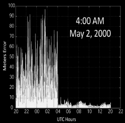
Historical Note: - Came about due to US “Selective Availability” (SA) - SA: Intentional GPS errors for security (civilians got degraded service) - SA turned off in May 2000 - DGPS still valuable for removing natural errors
1503.5 Advanced GPS Techniques
%% fig-cap: "Advanced GPS Techniques: A-GPS, RTK, and Signal Structure"
%% fig-alt: "Diagram showing three advanced GPS technologies"

%%{init: {'theme': 'base', 'themeVariables': { 'primaryColor': '#2C3E50', 'primaryTextColor': '#fff', 'primaryBorderColor': '#16A085', 'lineColor': '#16A085', 'secondaryColor': '#E67E22', 'tertiaryColor': '#ecf0f1', 'noteTextColor': '#2C3E50', 'noteBkgColor': '#fff3cd', 'textColor': '#2C3E50', 'fontSize': '16px'}}}%%

graph TB
    Advanced[Advanced GPS<br/>Techniques]

    Advanced --> AGPS[Assisted GPS<br/>A-GPS]
    Advanced --> RTK[Real-Time Kinematic<br/>RTK / Carrier Phase]
    Advanced --> Signal[Signal Structure<br/>Multi-frequency]

    AGPS --> A1[Problem:<br/>Ephemeris download<br/>~20s per satellite]
    A1 --> A2[Solution:<br/>Get ephemeris via<br/>cellular/Wi-Fi]
    A2 --> A3[Benefits:<br/>Faster TTFF<br/>Works indoors better]

    RTK --> R1[Carrier Phase<br/>Measurement<br/>λ = 19cm L1 band]
    R1 --> R2[Accuracy:<br/>2-5 cm<br/>centimeter-level!]
    R2 --> R3[Requirements:<br/>Continuous lock<br/>No cycle slips<br/>Initial ambiguity]
    R3 --> R4[Applications:<br/>Surveying<br/>Autonomous vehicles<br/>Precision agriculture]

    Signal --> S1[Multi-frequency:<br/>L1: 1575 MHz<br/>L2: 1227 MHz<br/>L5: 1176 MHz]
    S1 --> S2[Data Rate:<br/>Only 50 bps!<br/>Very slow]
    S2 --> S3[Spread Spectrum:<br/>CDMA<br/>Signal strength +<br/>interference resistance]

    style Advanced fill:#2C3E50,stroke:#16A085,stroke-width:4px,color:#fff
    style AGPS fill:#16A085,stroke:#2C3E50,stroke-width:3px,color:#fff
    style RTK fill:#E67E22,stroke:#16A085,stroke-width:3px,color:#fff
    style Signal fill:#16A085,stroke:#2C3E50,stroke-width:3px,color:#fff
    style R2 fill:#2C3E50,stroke:#16A085,stroke-width:3px,color:#fff
    style A3 fill:#16A085,stroke:#2C3E50,stroke-width:2px,color:#fff
1. Assisted-GPS (A-GPS): - Problem: Downloading ephemeris (satellite orbital data) takes ~20s per satellite - Solution: Get ephemeris via cellular or Wi-Fi data connection - Benefit: Faster Time To First Fix (TTFF), works indoors better
2. Carrier Phase Positioning (RTK): - GPS signal wavelength: ~19 cm (L1 band at 1575 MHz) - Measure phase of carrier wave (not just code) - Accuracy: Centimeter-level (2-5 cm) - Requirements: - Very accurate initial location - Observe satellites for extended period - Maintain continuous lock (no “cycle slips”) - Applications: Surveying, precision agriculture, autonomous vehicles
3. Signal Structure: - Multiple frequency bands: L1 (1575 MHz), L2 (1227 MHz), L5 (1176 MHz) - Data rate: Only 50 bits per second (very slow!) - Uses spread-spectrum (CDSS) for signal strength and interference resistance
1503.6 Practical Example: RTK GPS in Precision Agriculture
Understanding when augmentation (DGPS, RTK) is needed is critical for IoT system design. Let’s examine a real-world precision agriculture case where centimeter-level accuracy is mandatory.
ImportantCase Study: Autonomous Tractor Row Guidance
Problem: Modern farms use autonomous tractors for planting and harvesting. Crop rows are spaced 30-76 cm (12-30 inches) apart. Standard GPS (5-10 meter accuracy) would cause the tractor to:
- Destroy crops: Driving over planted rows instead of between them
- Miss coverage: Leaving gaps in planting or harvesting
- Overlap excessively: Wasting seeds, fertilizer, and fuel
Why Standard GPS Fails:
| Technology | Accuracy | Can Navigate 50cm Rows? | Result |
|---|---|---|---|
| Smartphone GPS | 5-10 m | No | 10× too imprecise—tractor wanders across 20 rows |
| DGPS | 0.5-1 m | No | Still 2× too large—damages crops on both sides |
| RTK GPS | 1-2 cm | Yes | Pass-to-pass accuracy maintains lane position |
Solution: RTK GPS provides sub-2cm accuracy enabling:
- Straight-line guidance: Maintain row centerline within ±2 cm over 1 km runs
- Repeat passes: Return to exact same tracks on subsequent operations (planting → spraying → harvesting)
- Nighttime operation: Autonomous 24/7 operation without visual references
- Reduced overlap: Typical 5-10% overlap reduced to 1-2% (saves $25,000-$50,000/year on 1000-acre farm in fuel, seeds, chemicals)
%% fig-cap: "RTK GPS System Architecture for Precision Agriculture"
%% fig-alt: "Diagram showing RTK GPS setup for autonomous tractor"

%%{init: {'theme': 'base', 'themeVariables': { 'primaryColor': '#2C3E50', 'primaryTextColor': '#fff', 'primaryBorderColor': '#16A085', 'lineColor': '#16A085', 'secondaryColor': '#E67E22', 'tertiaryColor': '#ecf0f1', 'noteTextColor': '#2C3E50', 'noteBkgColor': '#fff3cd', 'textColor': '#2C3E50', 'fontSize': '16px'}}}%%

graph TB
    subgraph Satellites["GPS Constellation"]
        S1[GPS Satellites<br/>L1: 1575 MHz<br/>L2: 1227 MHz]
    end

    subgraph Base["RTK Base Station - Farm Edge"]
        BS[Base Station<br/>Surveyed position<br/>Lat/Lon known to<br/>±1 cm accuracy]
        Calc[Calculate Carrier<br/>Phase Errors<br/>Real-time corrections]
    end

    subgraph Mobile["Autonomous Tractor"]
        Rover[RTK Rover Receiver<br/>Dual-frequency<br/>L1 + L2 carrier phase]
        Combine[Combine GPS +<br/>RTK Corrections<br/>Achieve 1-2 cm fix]
        Autopilot[Autopilot System<br/>Maintain row centerline<br/>±2 cm deviation]
    end

    subgraph Radio["Correction Transmission"]
        Link[Radio Link<br/>900 MHz or 2.4 GHz<br/>Range: 10 km<br/>Update rate: 1-10 Hz]
    end

    subgraph Field["Field Operations"]
        Rows[Crop Rows<br/>50-76 cm spacing<br/>1 km length]
        Result[Results:<br/>Zero crop damage<br/>1-2% overlap<br/>$40K/year savings]
    end

    S1 -->|GPS signals| BS
    S1 -->|GPS signals| Rover

    BS --> Calc
    Calc --> Link
    Link -.->|RTK corrections<br/>1-10 Hz updates| Rover

    Rover --> Combine
    Combine --> Autopilot
    Autopilot --> Rows
    Rows --> Result

    style BS fill:#16A085,stroke:#2C3E50,stroke-width:3px,color:#fff
    style Combine fill:#2C3E50,stroke:#16A085,stroke-width:3px,color:#fff
    style Result fill:#16A085,stroke:#2C3E50,stroke-width:3px,color:#fff
    style S1 fill:#2C3E50,stroke:#16A085,stroke-width:2px,color:#fff
    style Link fill:#E67E22,stroke:#16A085,stroke-width:2px,color:#fff
    style Rows fill:#E67E22,stroke:#2C3E50,stroke-width:2px,color:#fff
    style Autopilot fill:#E67E22,stroke:#16A085,stroke-width:2px,color:#fff
TipWhen to Choose RTK vs. DGPS vs. Standard GPS
Decision Framework for IoT Location Systems:
| Application Requirement | Recommended Technology | Typical Cost | Justification |
|---|---|---|---|
| Row-crop farming (30-76 cm rows) | RTK GPS | $15,000-$25,000 | 1-2 cm accuracy required; ROI in 1-2 years from reduced overlap |
| Broadcast fertilizing (no rows) | DGPS | $2,000-$5,000 | 0.5-1 m sufficient to avoid coverage gaps and excessive overlap |
| Livestock tracking (which pasture?) | Standard GPS | $50-$200 | 5-10 m accuracy adequate; just need geofence boundaries |
| Construction grading (±2 cm elevation) | RTK GPS + tilt sensors | $20,000-$40,000 | Vertical accuracy critical for drainage and leveling |
| Drone surveying (topographic maps) | RTK GPS or PPP | $5,000-$15,000 | Centimeter-level required for accurate 3D models |
| Fleet delivery tracking | Smartphone GPS | Free (built-in) | Know which city block vehicle is on; 5-10m sufficient |
Key Insight: Match accuracy to application—don’t over-engineer! RTK GPS costs 10-50× more than standard GPS. Only use it when centimeter-level precision delivers measurable ROI.
CautionRTK GPS Limitations in IoT Deployments
Common Pitfalls When Designing RTK Systems:
- Requires Continuous Radio Link (Base ↔︎ Rover):
- Problem: Hills, trees, buildings block 900 MHz/2.4 GHz radio
- Range limit: Typically 10 km line-of-sight, much less in rugged terrain
- Solution: Deploy multiple base stations or use NTRIP (internet-based corrections)
- Loses Accuracy if Satellite Lock Breaks:
- Problem: Driving under trees, bridges, or in narrow canyons causes “cycle slips”
- Recovery time: 30 seconds to several minutes to re-establish centimeter fix
- Fallback: System degrades to DGPS (1m) or standard GPS (5-10m) during outages
- Expensive and Power-Hungry:
- Base station: 5-15 watts continuous power (requires AC or large solar panel)
- Rover receiver: 2-5 watts (vs. 0.5W for standard GPS)
- Total system cost: $15,000-$25,000 (base + rover + radio + installation)
- Requires Expertise to Set Up:
- Base station must be surveyed to ±1 cm accuracy (professional surveyor)
- Radio frequency coordination (avoid interference with other farm equipment)
- Antenna placement (clear sky view, stable mounting, lightning protection)
When RTK is NOT Worth It: - Wrong: Use RTK to track shipping containers (5-10m GPS sufficient to know “which warehouse”) - Wrong: Track hospital wheelchairs indoors (GPS doesn’t work indoors; use BLE beacons instead) - Right: Autonomous tractors planting 50cm rows ($40,000/year savings justifies $20,000 equipment)
1503.7 Knowledge Check
1503.8 What’s Next
Continue to Indoor Positioning Technologies to learn about Wi-Fi fingerprinting, BLE beacons, UWB, and sensor fusion techniques for positioning where GPS signals cannot reach.