710 RPL Production Framework and Summary
By the end of this section, you will be able to:
- Understand production RPL framework architecture
- Analyze RPL performance trade-offs for real deployments
- Apply RPL concepts to large-scale IoT deployments
- Summarize key RPL concepts for practical implementation
710.1 Prerequisites
Before diving into this chapter, you should be familiar with:
- RPL Introduction and Core Concepts: Understanding DODAG topology, RANK mechanism, and why RPL is needed for IoT
- RPL DODAG Construction and Modes: Knowledge of how DODAGs are built and the differences between Storing and Non-Storing modes
- RPL Traffic Patterns and Design: Traffic patterns, memory requirements, and network design
This Series: - RPL Introduction - Core concepts and fundamentals - RPL DODAG Construction and Modes - Building DODAGs and routing modes - RPL Traffic Patterns and Design - Traffic patterns and network design lab - RPL Production and Summary - This chapter
Hands-On: - RPL Production and Review - Storing vs Non-Storing mode deployment - Simulations Hub - Test RPL DODAG formation in simulators
710.2 Production RPL Framework
This section provides a comprehensive production-ready Python framework for RPL (IPv6 Routing Protocol for Low-Power and Lossy Networks), including DODAG construction, RANK calculation, Trickle timer, and both Storing and Non-Storing modes.
710.2.1 Framework Architecture
This production framework provides comprehensive RPL protocol capabilities:
- DODAG Construction: Distance-vector routing with RANK-based hierarchy, automatic parent selection
- Trickle Timer: RFC 6206 implementation for adaptive DIO transmission (Imin to Imax intervals)
- Routing Modes: Storing mode with distributed routing tables, non-storing mode support
- Objective Functions: OF0 (hop count), MRHOF (ETX), Energy, Latency-based routing
- Loop Prevention: RANK mechanism prevents routing loops, acyclic graph guaranteed
- Control Messages: DIO (DODAG Information), DAO (Destination Advertisement), DIS, DAO-ACK
- Traffic Patterns: Upward (many-to-one), downward (one-to-many), point-to-point routing
- Network Repair: DODAG version increment for global topology changes
- Parent Selection: Preferred parent with backup parent set for reliability
The framework demonstrates production-ready patterns for IPv6-based IoT networks with comprehensive statistics tracking, realistic link metrics, and complete DODAG lifecycle management.
710.3 Key Concepts
- DODAG (Destination Oriented Directed Acyclic Graph): Tree topology with single root; all upward paths lead to root
- RANK: Hierarchical position in DODAG; prevents routing loops, enables parent selection
- Distance-Vector Routing: Each node knows next hop (parent), not entire network topology
- Objective Function: Algorithm for selecting best parent (hop count, energy, ETX); pluggable for different metrics
- Parent Selection: Preferred parent with backup parents for fault tolerance
- DIO (DODAG Information Object): Control message advertising DODAG topology; triggers parent selection
- DAO (Destination Advertisement Object): Backward routing information in Storing mode for downward paths
- Storing vs Non-Storing: Storing mode caches routes on each node (optimal paths, more memory); Non-Storing centralizes at root (source routing)
- IPv6-Based: Native IPv6 protocol running over 6LoWPAN on IEEE 802.15.4 networks
- Loop Prevention: DAG property and RANK mechanism guarantee acyclic routing, preventing loops
- Many-to-One Traffic: Optimized for sensor networks where all data flows toward root gateway
- Multiple Instances: Different RPL instances on same network support different applications/metrics
- Lossy Link Support: Designed for 10-40% packet loss typical in wireless sensor networks
- Scalability: Non-Storing mode scales to thousands of nodes; Storing mode optimizes for smaller networks
- Control Message Types: DIO, DAO, DIS, DAO-ACK enable DODAG construction, topology updates, and route advertisement
710.4 Visual Reference Gallery
Explore these AI-generated visualizations that illustrate RPL routing concepts.

DODAG construction progresses outward from the root as each layer of nodes calculates RANK and propagates DIO messages.

A complete DODAG provides reliable upward routing for all sensor data to reach the root gateway.

RPL’s architecture integrates multiple components to provide efficient routing for constrained IoT networks.

Understanding how RPL combines distance-vector simplicity with advanced features helps contextualize its design decisions.
710.5 Chapter Summary
RPL (IPv6 Routing Protocol for Low-Power and Lossy Networks) is the IETF standard routing protocol designed specifically for IPv6-based IoT networks with resource-constrained devices, lossy wireless links, and convergent traffic patterns.
Unlike traditional routing protocols (OSPF, RIP) designed for wired networks with powerful routers, RPL addresses IoT’s unique challenges: - Limited resources: Sensors have <32 KB RAM, limited CPU, battery power - Lossy links: Wireless links lose 10-40% of packets; unreliable compared to wired networks - Traffic patterns: Most data flows toward a root gateway (convergent/many-to-one pattern), not uniformly across network - Multiple metrics: Performance depends on energy, latency, reliability - not just hop count
DODAG (Destination Oriented Directed Acyclic Graph) is RPL’s core concept. Instead of a full routing table, each node stores only its preferred parent(s). The DODAG forms a tree with a single root (typically the gateway). All upward paths eventually lead to root through parent pointers, creating a loop-free graph by design.
RANK is the hierarchical position in the DODAG. Root has RANK 0. Each node calculates its RANK based on parent’s RANK plus a metric. RANK enforces hierarchy - nodes never forward packets to higher-ranked nodes, preventing loops. This is simpler than count-to-infinity prevention used in traditional distance-vector protocols.
Parent selection is flexible. RPL computes the Objective Function (OF) - an algorithm combining multiple metrics (hop count, energy, ETX) to select the best parent. The protocol includes: - Objective Function Zero (OF0): Simple hop count minimization - Minimum Rank with Hysteresis Objective Function (MRHOF): Considers link quality (ETX) with hysteresis to prevent rapid parent switches
Nodes maintain a preferred parent (primary) and backup parent set for resilience. When preferred parent fails, nodes can quickly switch to backup, enabling self-healing mesh networks.
Control messages are ICMPv6-based: - DIO (DODAG Information Object): Root advertises DODAG; nodes forward DIO when joining DODAG. Contains RANK, Objective Function, DODAG ID - DIS (DODAG Information Solicitation): Orphaned node requests DODAG information to join network - DAO (Destination Advertisement Object): Node advertises reachability to upstream nodes (for downward routing in Storing mode) - DAO-ACK: Acknowledgment of DAO receipt
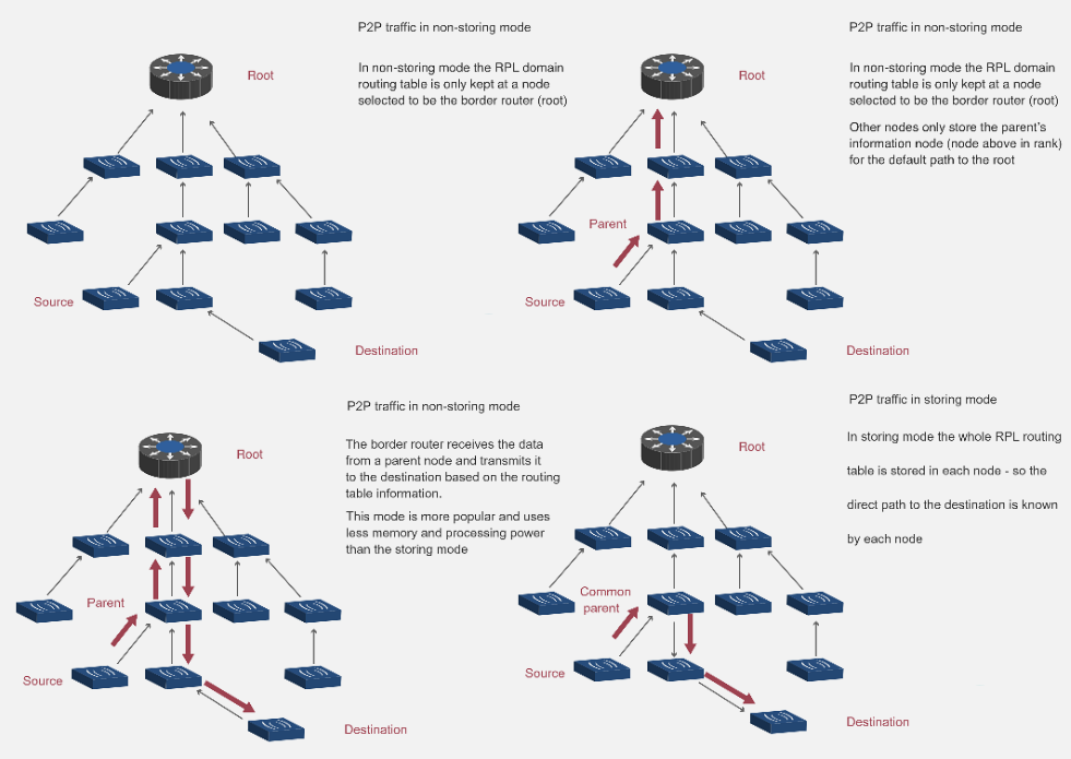
Two operational modes: 1. Storing mode: Each node caches routing table with paths to other nodes; enables optimal point-to-point paths but requires more memory 2. Non-Storing mode: Each node stores only parent pointer; downward routes use source routing (root specifies full path); saves memory
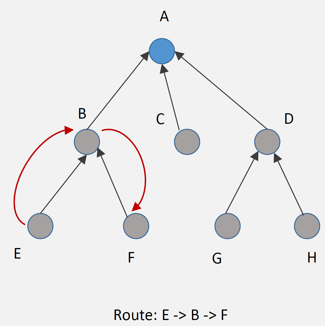
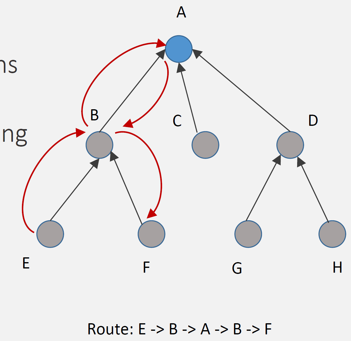
Upward routing (sensors to root) is identical in both modes: each node sends to parent. Downward routing (root to sensors) differs: Storing mode uses cached routes, Non-Storing uses source routing from root. Point-to-point routing (sensor to sensor) uses upward path to common ancestor then downward path in Storing mode, or via root in Non-Storing mode.
Traffic patterns RPL optimizes for: - Many-to-one: Sensors report to gateway (most common); both modes identical - One-to-many: Gateway commands actuators; Storing better (optimal paths), Non-Storing uses source routing - Point-to-point: Device-to-device communication; Storing can optimize, Non-Storing routes via root
DODAG construction follows a multi-step process: 1. Root node sends DIO with RANK=0, establishes DODAG ID 2. Nodes receive DIO, calculate their own RANK, select preferred parent 3. Nodes send own DIO to propagate DODAG downward 4. Upward routes form automatically (parent pointers) 5. In Storing mode, nodes send DAO to advertise reachability upward 6. Downward routes created from DAO information
Network repair occurs when topology changes (links fail, nodes join/leave). RPL detects changes via loss of DIO from parent. Upon failure, node can quickly switch to backup parent. Global repairs happen via DODAG version increment from root.
Performance characteristics: - Memory: Non-Storing mode uses ~40% less network-wide memory - Latency: Storing mode better for point-to-point (optimal paths); identical for many-to-one - Scalability: Non-Storing scales better (limited by root CPU, not node memory); can handle thousands of nodes - Convergence: Faster than traditional distance-vector protocols; parent selection avoids count-to-infinity delays
Why RPL dominates IoT: - Standardized by IETF (RFC 6550, 2012) - Native IPv6, works with 6LoWPAN compression - Handles lossy, low-power networks inherently - Flexible metrics through pluggable Objective Functions - Proven in real-world deployments (Thread, many Zigbee implementations) - Works at Layer 3, protocol-agnostic at Link Layer (works over 802.15.4, Wi-Fi, etc.)
Use cases: - Smart home sensor networks (temperature, humidity, motion) - Industrial IoT monitoring (machines, energy, safety) - Smart city deployments (street lights, parking sensors, environmental monitoring) - Building automation (HVAC, lighting, access control) - Agriculture IoT (soil moisture, weather stations) - Any IPv6-based constrained network requiring self-healing mesh
710.6 Original Source Figures (Alternative Views)
The following figures from the CP IoT System Design Guide provide alternative visual representations of RPL operation concepts covered in this chapter.
Source: CP IoT System Design Guide, Chapter 4 - Routing
Source: CP IoT System Design Guide, Chapter 4 - Routing
Source: CP IoT System Design Guide, Chapter 4 - Routing
710.7 What’s Next
Now that you understand RPL’s design for IoT-specific routing, the next sections explore other specialized protocols and practical network design that applies routing concepts.
Upcoming topics: - Transport protocols: TCP vs UDP choice affects routing (TCP assumes persistent paths) - Network topologies: How RPL builds different topologies (tree, mesh, hybrid) - Design implications: Choosing between routing protocols based on network characteristics - Wireless technologies: How Wi-Fi, BLE, and other physical layers integrate with routing - Protocol selection: Matching protocols to IoT scenarios
The DODAG, parent selection, and metric optimization concepts from RPL apply broadly to understanding how specialized IoT protocols work and when to deploy them.
710.8 Summary
RPL (IPv6 Routing Protocol for Low-Power and Lossy Networks) is the standard routing protocol for IoT:
Core Concepts: - DODAG: Destination Oriented Directed Acyclic Graph (tree toward root) - RANK: Hierarchical position (prevents loops, enables upward routing) - Distance-Vector: Each node knows next hop (parent), not entire network - IPv6-based: Works with 6LoWPAN for constrained devices
Why Not Traditional Routing: - Resource constraints: IoT devices lack CPU, RAM, power for OSPF/RIP - Multiple metrics: RPL supports flexible objective functions (latency, energy, ETX) - Multiple instances: Different routing for different applications on same network - Lossy links: RPL designed for 10-40% packet loss - Traffic patterns: Optimized for many-to-one (sensors to gateway)
Control Messages (ICMPv6): - DIO: DODAG Information Object (advertise DODAG) - DIS: DODAG Information Solicitation (request DODAG info) - DAO: Destination Advertisement Object (advertise reachability) - DAO-ACK: DAO Acknowledgment (confirm receipt)
Routing Modes: - Storing: Distributed routing tables (optimal paths, higher memory) - Non-Storing: Centralized routing at root (source routing, lower memory)
Traffic Patterns: - Many-to-One (upward): Sensors to Root (most common, both modes identical) - One-to-Many (downward): Root to Actuators (Storing optimal, Non-Storing via source routing) - Point-to-Point: Sensor to Sensor (Storing can optimize, Non-Storing via root)
DODAG Construction: 1. Root sends DIO (RANK 0, DODAG ID) 2. Nodes receive DIO, calculate RANK, select parent 3. Nodes send DIO (propagate DODAG) 4. Upward routes automatic (parent pointers) 5. Downward routes via DAO (Storing mode)
Loop Prevention: - DAG property: Acyclic by definition - RANK mechanism: Enforces hierarchy, prevents routing to higher RANK - No count-to-infinity: RANK bounds prevent infinite loops
Mode Selection: - Storing: Devices with >32 KB RAM, low latency needed, P2P common - Non-Storing: Battery devices <16 KB RAM, many-to-one primary, large networks
Performance: - Memory: Non-Storing ~40% less network-wide - Latency: Storing better for P2P, identical for many-to-one - Scalability: Non-Storing scales to more nodes (limited by root, not node memory)
Use Cases: - Smart home sensor networks (temperature, motion) - Industrial IoT monitoring - Smart city deployments (street lights, parking) - Building automation - Any IPv6-based constrained network (6LoWPAN, Thread)
Standards: - RFC 6550: RPL specification (IETF, 2012) - RFC 6552: Objective Function Zero (OF0, hop count) - RFC 6719: Minimum Rank with Hysteresis Objective Function (MRHOF)
RPL is the de facto standard for routing in IPv6-based IoT networks, providing efficient, scalable routing optimized for resource-constrained devices in lossy networks with convergent traffic patterns.