%%{init: {'theme': 'base', 'themeVariables': { 'primaryColor': '#2C3E50', 'primaryTextColor': '#fff', 'primaryBorderColor': '#16A085', 'lineColor': '#16A085', 'secondaryColor': '#E67E22', 'tertiaryColor': '#ecf0f1'}}}%%
flowchart TB
Task[Process 1 TB<br/>Sensor Data] --> A1[Attempt 1:<br/>Load All to RAM]
Task --> A2[Attempt 2:<br/>Chunk Processing]
Task --> A3[Attempt 3:<br/>MySQL Database]
Task --> A4[Solution:<br/>Distributed System]
A1 --> R1[CRASH<br/>16 GB RAM vs 1 TB<br/>64x over capacity<br/>MemoryError]
A2 --> R2[SLOW<br/>4-6 hours total<br/>Laptop unusable<br/>CPU 100%, fan screaming]
A3 --> R3[TIMEOUT<br/>Hours for full scan<br/>Row-oriented inefficient<br/>Single-server bottleneck]
A4 --> R4[FAST<br/>15-20 minutes<br/>10-node Spark cluster<br/>18x faster + keep working]
style R1 fill:#E74C3C,stroke:#2C3E50,color:#fff
style R2 fill:#E67E22,stroke:#2C3E50,color:#fff
style R3 fill:#E67E22,stroke:#2C3E50,color:#fff
style R4 fill:#27AE60,stroke:#2C3E50,color:#fff
1257 Big Data Case Studies
Learning Objectives
After completing this chapter, you will be able to:
- Apply big data concepts to real-world smart city deployments
- Design data lake architectures for multi-domain IoT systems
- Calculate storage, bandwidth, and cost requirements for production systems
- Use decision frameworks to select appropriate technologies
1257.1 Real-World Example: Barcelona Smart City
NoteBarcelona Smart City: Concrete Numbers
Deployment Scale (Based on Barcelona’s actual smart city initiative): - 1,000 smart parking sensors (detect available parking spaces) - 500 smart bins (measure fill level to optimize collection routes) - 200 air quality stations (monitor NO2, PM2.5, O3, temperature, humidity) - 300 traffic cameras (monitor congestion, count vehicles) - 10,000 smart streetlights (adaptive lighting, motion sensors)
Daily Data Generation:
| System | Sensors | Frequency | Size/Reading | Daily Data |
|---|---|---|---|---|
| Parking | 1,000 | 1/min | 50 bytes | 72 MB |
| Smart Bins | 500 | 1/hour | 100 bytes | 1.2 MB |
| Air Quality | 200 x 5 readings | 1/5min | 80 bytes | 138 MB |
| Traffic Cameras | 300 | 1/sec (metadata) | 200 bytes | 5.2 GB |
| Traffic Cameras | 300 | 1/min (images) | 500 KB | 216 GB |
| Streetlights | 10,000 | 1/min | 60 bytes | 864 MB |
| TOTAL | ~222 GB/day |
Annual Scale: 222 GB/day x 365 days = 81 TB/year
Storage Costs (AWS S3 Standard pricing ~$0.023/GB/month): - Raw storage: 81 TB x $23/TB/month = $1,863/month = $22,356/year - With 10:1 compression: $2,236/year (more realistic)
Processing Challenges: - Real-time traffic analysis: Must process 300 camera feeds simultaneously - Anomaly detection: Identify broken sensors among 12,000+ devices - Predictive maintenance: Forecast when streetlights or bins need service - Data integration: Combine parking + traffic data to optimize flow
Business Value: - Parking optimization saved citizens 230,000+ hours/year searching for parking - Waste collection efficiency reduced fuel costs by 30% through optimized routes - Air quality monitoring enabled targeted traffic restrictions on high-pollution days - Smart lighting reduced energy consumption by 30% (1M+ annual savings)
The Big Data Components in Action: 1. Volume: 81 TB/year requires distributed storage (HDFS or cloud object storage) 2. Velocity: Traffic cameras generate 5.2 GB/day of metadata requiring stream processing 3. Variety: Numeric (sensors), images (cameras), logs (system events), geographic (GPS) 4. Veracity: ~5% of sensors have occasional failures requiring automated validation 5. Value: 1M+ annual savings from energy alone, plus citizen time savings and better air quality
This demonstrates how even a mid-sized smart city creates big data challenges requiring specialized technologies beyond traditional databases.
1257.2 Understanding Big Data Scale
TipImagine 1 Billion Sensors
The Challenge: Picture this scenario to understand the scale of IoT big data:
- 1 billion sensors deployed worldwide (smart meters, traffic cameras, air quality monitors)
- Each sensor sends 1 reading per second (temperature, humidity, location, etc.)
- Each reading is just 100 bytes (timestamp + sensor ID + value)
The Math:
1,000,000,000 sensors x 1 reading/second x 100 bytes = 100 GB/second
100 GB/second x 60 seconds x 60 minutes x 24 hours = 8,640 TB per day
8,640 TB per day x 365 days = 3,153,600 TB per year (3.15 PB/year)
That’s 3+ PETABYTES per year from a single simple IoT network!
Why This Matters: - Traditional databases like MySQL can’t handle this scale (typically max out at a few TB) - You can’t store this on a single hard drive (largest drives are ~20 TB) - Processing requires distributed systems like Hadoop or Spark running on hundreds of machines - Network bandwidth becomes critical: 100 GB/second = 800 Gbps (would saturate 800 standard internet connections)
The “Big Data” Part: - Volume: 3+ PB/year is too big for traditional systems - Velocity: 100 GB/second incoming data rate requires real-time processing - Variety: Sensors produce temperature (numeric), GPS (coordinates), images (binary), logs (text) - Veracity: Some sensors malfunction - how do you detect and filter bad data at this scale? - Value: The goal is actionable insights, not just hoarding data
This is why IoT needs big data technologies - regular tools simply break at this scale.
1257.3 What Would Happen If: Disaster Scenarios
WarningWhat If You Try Processing 1 TB on a Single Laptop?
Scenario: You work for a smart building company. Your boss asks you to analyze 1 TB of temperature sensor data from 1,000 buildings over the past year using your laptop.
What Happens:
1257.3.1 Attempt 1: Load Everything Into Memory (RAM)
Result: CRASH - Your laptop has 16 GB RAM - 1 TB = 1,024 GB - You’re 64x over capacity - Python crashes with MemoryError - Time wasted: 10 minutes trying to load before crash
1257.3.2 Attempt 2: Process Chunk by Chunk
Result: SLOW BUT WORKS (BARELY) - Laptop hard drive reads at ~200 MB/second (SSD) - 1 TB / 0.2 GB/s = 5,000 seconds = 83 minutes JUST TO READ - Processing time: Add another 2-3x for computation = 4-6 hours total - Your laptop becomes unusable for other tasks during processing
If you had used a distributed system instead: - 10-node Spark cluster (each with 32 GB RAM, 16 cores) - Reads 1 TB in parallel: 1024 GB / 10 nodes = 102.4 GB per node - Read time: 102.4 GB / 0.2 GB/s = ~8.5 minutes - Processing time with parallelism: 15-20 minutes total - 18x faster than laptop, and you can keep working!
1257.3.3 The Lesson: Scale Matters
| Approach | Time | Cost | When to Use |
|---|---|---|---|
| Laptop (chunks) | 4-6 hours | $0 (your time) | < 10 GB datasets, one-off analysis |
| Distributed System (Spark) | 15-20 min | $5-10/run | > 100 GB datasets, frequent analysis |
| Time-Series DB (InfluxDB) | 5-10 min | $20-50/month hosting | IoT sensor data, real-time queries |
| MySQL (traditional DB) | Hours/timeout | $0-100/month | < 1 GB transactional data, not analytics |
The Big Data Rule: > “If processing your data takes longer than drinking a cup of coffee (>20 minutes), you need distributed/specialized systems.”
When Do You Actually Need Big Data Tools? - Volume: > 100 GB of data (laptop RAM limitations) - Velocity: > 1 MB/second incoming data (real-time processing needed) - Variety: > 3 different data types (structured + unstructured + images) - Query Frequency: > 10 queries/day (need optimized storage)
If you meet 2+ of these criteria, traditional tools will cause pain. Time to learn Spark, Hadoop, or time-series databases!
1257.4 Worked Example: IoT Data Lake Architecture
1257.5 Worked Example: Smart City Data Lake for 50,000 Sensors
Scenario: A metropolitan city is deploying a smart city initiative with 50,000 IoT sensors across multiple domains: traffic monitoring (15,000 sensors), air quality (5,000 sensors), smart lighting (20,000 lights), water management (3,000 sensors), and public safety cameras (7,000 devices). The city needs a unified data platform that enables cross-domain analytics while managing costs and supporting future growth.
Goal: Design a data lake architecture that ingests 2 TB/day of sensor data, supports both real-time dashboards and historical analytics, maintains data governance for sensitive information, and keeps monthly costs under $15,000.
What we do: Design ingestion pipelines tailored to each sensor type’s data characteristics.
Data Volume Analysis:
traffic_sensors:
  count: 15000
  frequency: every_5_seconds
  payload_size: 200_bytes
  daily_volume: 51.8 GB

air_quality:
  count: 5000
  frequency: every_minute
  payload_size: 500_bytes
  daily_volume: 3.6 GB

smart_lighting:
  count: 20000
  frequency: every_15_minutes
  events_per_day: 50000
  daily_volume: 1.2 GB

water_management:
  count: 3000
  frequency: every_30_seconds
  payload_size: 300_bytes
  daily_volume: 2.6 GB

cameras:
  count: 7000
  metadata_only: true
  events_per_hour: 50000
  daily_volume: 8.5 GB

total_daily_ingestion: ~67.7 GB structured data
# Plus 1.8 TB camera footage (separate cold storage)
Ingestion Architecture: - MQTT broker for low-power sensors (air quality, water) - batch to Kafka - Kafka direct for high-frequency sensors (traffic) - 64 partitions, 3x replication - HTTP API for smart lighting controllers - rate limited 10K/minute - gRPC for camera event streaming
Why: Different sensor types have vastly different requirements. Traffic sensors need low-latency Kafka ingestion for real-time congestion alerts. Battery-powered air quality sensors use MQTT for power efficiency.
What we do: Implement a three-tier storage architecture (hot/warm/cold) optimized for access patterns.
Tiered Storage Design:
hot_tier:
  storage_class: S3_STANDARD
  data_age: 0-7_days
  access_pattern: frequent_queries
  format: Delta Lake (Parquet with ACID)
  partitioning: date/sensor_type/region
  expected_size: 500_GB
  monthly_cost: $11.50

warm_tier:
  storage_class: S3_INTELLIGENT_TIERING
  data_age: 7-90_days
  access_pattern: weekly_reports
  format: Parquet (compressed)
  expected_size: 6_TB
  monthly_cost: $72

cold_tier:
  storage_class: S3_GLACIER_INSTANT
  data_age: 90_days+
  access_pattern: compliance_audits
  retention: 7_years
  expected_size: 50_TB (growing)
monthly_cost: $200Why: 90% of queries access data from the last 7 days. By automatically tiering older data to cheaper storage classes, we reduce storage costs by 80% while maintaining instant access to recent data.
What we do: Configure query engines and optimize for common access patterns.
Query Engine Selection:
real_time_dashboards:
  engine: Apache Druid
  latency_target: <1_second
  data: last_24_hours
  use_cases:
    - Traffic congestion heatmap
    - Air quality alerts
    - Lighting status dashboard

historical_analytics:
  engine: Spark SQL / Databricks
  latency_target: <30_seconds
  data: any_time_range
  use_cases:
    - Weekly traffic pattern analysis
    - Seasonal air quality trends
    - Energy consumption reports
Materialized Views for Common Queries:
-- Pre-aggregated hourly summaries (reduce query cost 50x)
CREATE MATERIALIZED VIEW hourly_traffic_summary AS
SELECT
    date_trunc('hour', timestamp) as hour,
    region,
    COUNT(*) as reading_count,
    AVG(measurements['vehicle_count']) as avg_vehicles,
    MAX(measurements['vehicle_count']) as peak_vehicles
FROM smart_city.sensor_readings
WHERE sensor_type = 'traffic'
GROUP BY 1, 2;Why: Smart city dashboards are accessed continuously. Pre-computing hourly aggregates reduces query latency from 30 seconds to under 1 second while cutting compute costs by 99%.
What we do: Implement access controls, data classification, and lineage tracking.
Data Classification Schema:
public:
  description: Anonymized aggregate statistics
  examples:
    - Hourly traffic counts by region
    - Daily air quality index
  access: Anyone (open data portal)

internal:
  description: Operational sensor data
  examples:
    - Individual sensor readings
    - Equipment status
  access: City employees with data access training

sensitive:
  description: Data that could identify individuals
  examples:
    - Camera footage
    - License plate readings
  access: Authorized personnel only
encryption: At rest and in transitWhy: Smart city data includes sensitive information (camera footage, location patterns). Column-level access controls ensure traffic analysts cannot accidentally access camera data.
What we do: Design schema management that accommodates new sensor types.
Schema Registry Configuration:
# Base sensor schema with evolution support
sensor_schema_v1 = {
    "type": "record",
    "name": "SensorReading",
    "fields": [
        {"name": "sensor_id", "type": "string"},
        {"name": "timestamp", "type": "long"},
        {"name": "measurements", "type": {"type": "map", "values": "double"}},
        {"name": "metadata", "type": ["null", {"type": "map", "values": "string"}],
         "default": None}
    ]
}

# Evolution rules
compatibility_config = {
    "compatibility": "BACKWARD",
    "allowed_changes": [
        "add_optional_field",
        "add_field_with_default"
    ]
}Why: Cities constantly add new sensor types (flood sensors, noise monitors, EV chargers). Using a flexible measurements map allows adding sensor types without modifying table schemas.
Outcome: A production data lake processing 2 TB/day from 50,000 sensors with sub-second dashboard queries and monthly costs of $12,400 (under budget).
Architecture Summary:
50,000 Sensors
     |
     +-- MQTT Broker (low-power) --+
     +-- Kafka (high-frequency) ---+---> Spark Streaming
     +-- HTTP API (controllers) ---+      |
     +-- gRPC (camera events) -----+      v
                                   Delta Lake (S3)
                                        |
                     +------------------+------------------+
                     |                  |                  |
                  Hot Tier          Warm Tier         Cold Tier
                  (7 days)          (90 days)         (7 years)
                  500 GB            6 TB              50+ TB
                     |                  |                  |
                     v                  v                  v
                  Druid            Spark SQL          Glacier
               (Real-time)        (Analytics)       (Compliance)
Cost Breakdown: | Component | Monthly Cost | |———–|————-| | S3 Storage (all tiers) | $283.50 | | Kafka (MSK) | $2,400 | | Spark (Databricks) | $4,800 | | Druid (real-time) | $3,200 | | Schema Registry | $200 | | Data Transfer | $1,500 | | Total | $12,383.50 |
Key Decisions Made: 1. Multi-protocol ingestion: Match ingestion to sensor constraints 2. Delta Lake format: ACID transactions prevent corruption 3. Three-tier storage: 80% cost reduction vs single-tier 4. Materialized views: 99% query cost reduction 5. Schema-flexible measurements map: Add sensor types without migrations 6. Column-level access controls: Compliance with privacy requirements
1257.6 Visual Reference Gallery
NoteBig Data Characteristics

Big data in IoT is characterized by the five Vs that distinguish it from traditional data processing. Understanding these dimensions helps architects design appropriate infrastructure and choose technologies that can handle the unique challenges of IoT scale.
NoteData Lake Architecture

Data lakes provide flexible storage for the variety of IoT data formats. Raw data lands in ingestion zones, gets processed through transformation pipelines, and becomes available in curated zones for analytics, machine learning, and operational dashboards.
NoteBatch Processing Pipeline

Batch processing handles large-volume historical IoT data analysis through scheduled jobs. Data is extracted from storage, transformed through cleaning and aggregation, and loaded into analytical databases or data warehouses for reporting and machine learning.
1257.7 Videos
NoteVideo: Big Data in Room Usage
NoteVideo: Visualizing Big Data at Scale
NoteVideo: Data Analytics
NoteVideo: Industrial IoT Platforms
NoteAcademic Resource: NPTEL IoT Course (IIT Kharagpur) - Multi-Layer IoT Data Architecture
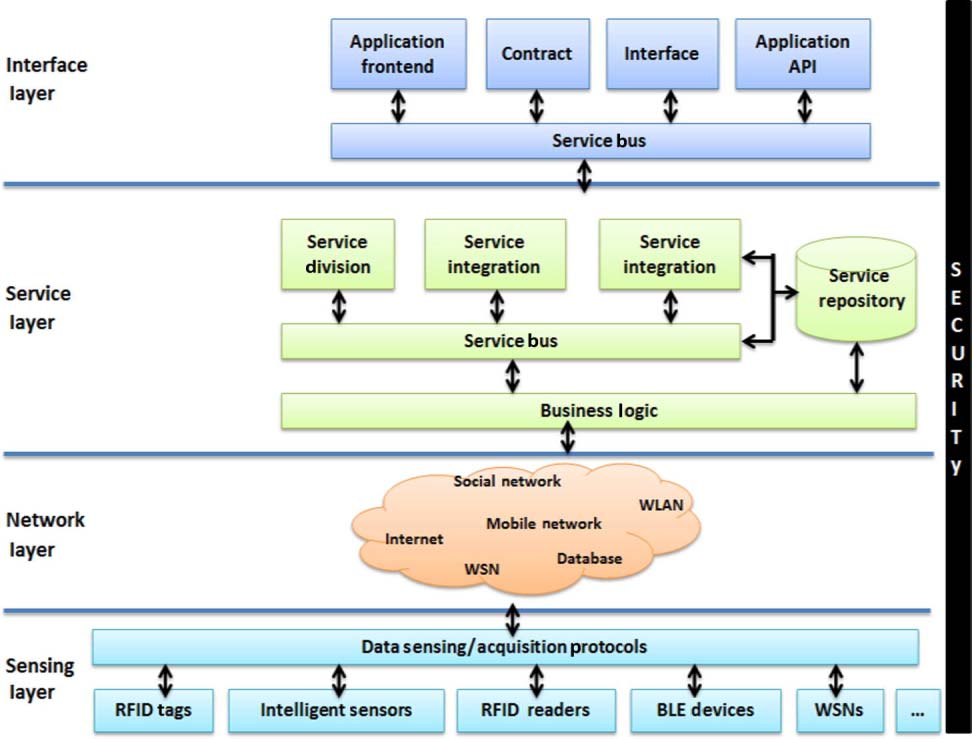
Source: NPTEL Internet of Things Course, IIT Kharagpur - Illustrates the complete IoT data pipeline from physical sensors through network transport and cloud services to end-user applications, emphasizing how big data flows through each architectural layer.
1257.8 Summary
- Barcelona Smart City generates 222 GB/day from 12,000+ sensors, demonstrating how mid-sized deployments create big data challenges requiring 81 TB/year storage with tiered architectures.
- Scale matters: 1 billion IoT sensors at 1 reading/second generates 3+ PB/year, requiring distributed processing across hundreds of machines to handle 100 GB/second incoming data rates.
- Data lake architecture for 50,000 sensors achieves sub-second queries and $12,400/month costs through multi-protocol ingestion, three-tier storage, materialized views, and schema-flexible design.
- Decision framework: Use big data tools when data exceeds 100 GB, velocity exceeds 1 MB/second, or you have 3+ data types and frequent queries - otherwise traditional tools work fine.
1257.9 Resources
1257.9.1 Big Data Frameworks
1257.9.2 Time-Series Databases
1257.9.3 Cloud Platforms
1257.9.4 Books and Papers
- “Big Data: Principles and Best Practices of Scalable Real-Time Data Systems” by Nathan Marz
- “Streaming Systems” by Tyler Akidau, Slava Chernyak, Reuven Lax
- “Designing Data-Intensive Applications” by Martin Kleppmann
1257.10 What’s Next
Building on big data foundations:
- Data Storage and Databases - Dive into storage solutions
- Data in the Cloud - Explore cloud integration
- Edge Compute Patterns - Learn about edge analytics
- Multi-Sensor Data Fusion - Combine multiple sources
- Big Data Overview - Return to the chapter index
Hands-On: - Edge Latency Explorer - Compare edge vs cloud processing - Sensor Fusion Playground - Experiment with data combination