%% fig-cap: "S-MAC Frame Structure showing synchronized duty cycling"
%% fig-alt: "Gantt chart showing S-MAC frame structure with Node A and Node B synchronized through SYNC, RTS/CTS, DATA, and SLEEP phases"
%%{init: {'theme': 'base', 'themeVariables': {'primaryColor': '#2C3E50', 'primaryTextColor': '#fff', 'primaryBorderColor': '#1a252f', 'lineColor': '#16A085', 'secondaryColor': '#16A085', 'tertiaryColor': '#E67E22'}}}%%
gantt
    title S-MAC Frame Structure
    dateFormat X
    axisFormat %s

    section Node A
    SYNC     :a1, 0, 1
    RTS/CTS  :a2, 1, 2
    DATA     :a3, 2, 4
    SLEEP    :a4, 4, 10

    section Node B
    SYNC     :b1, 0, 1
    RTS/CTS  :b2, 1, 2
    DATA     :b3, 2, 4
    SLEEP    :b4, 4, 10
370 Energy Management and Duty Cycling
370.1 Learning Objectives
By the end of this chapter, you will be able to:
- Analyze energy consumption profiles: Quantify power draw across radio, sensing, processing, and sleep states
- Apply conservation strategies: Implement duty cycling, data reduction, and topology control techniques
- Compare MAC protocols: Evaluate S-MAC (synchronous) vs B-MAC/X-MAC (asynchronous) duty cycling
- Design energy-aware systems: Balance trade-offs between energy, latency, reliability, and throughput
- Calculate network lifetime: Use FND, HND, and LND metrics for deployment planning
- Evaluate energy harvesting: Determine when harvesting outperforms battery-only solutions
370.2 Characteristics of Sensor Systems
Sensor systems encompass the complete stack from physical sensing to data interpretation, with characteristics that determine their effectiveness and applicability.
370.2.1 System-Level Characteristics
Scalability: Ability to function effectively as network size grows from tens to thousands of nodes.
Challenges: - Routing complexity increases with node count - Data aggregation and processing load - Network management and configuration - Address space and identifier management
Solutions: - Hierarchical architectures (clustering) - Scalable routing protocols (geographic, hierarchical) - Distributed data aggregation - Self-organizing capabilities
Reliability: Ensuring consistent operation despite node failures, communication errors, and environmental challenges.
Approaches: - Redundancy: Multiple sensors measuring same phenomenon - Multi-path routing: Alternative communication paths - Fault detection and recovery mechanisms - Data validation and error correction
Robustness: Operating effectively under varying conditions, interference, and unexpected events.
Techniques: - Adaptive protocols adjusting to conditions - Interference mitigation - Environmental calibration - Graceful degradation under stress
Latency: Time between event occurrence and system response or user notification.
Factors: - Sensing frequency and processing time - Multi-hop routing delays - Gateway processing and cloud transmission - Application-specific requirements (real-time vs. batch)
Accuracy and Precision: Quality of measurements and consistency of readings.
Considerations: - Sensor calibration and drift - Environmental interference - Data fusion from multiple sensors - Trade-offs with power consumption
370.2.2 Network Characteristics
Topology: Physical and logical arrangement of nodes.
Common Topologies: - Star: Nodes communicate directly with central gateway - Tree/Hierarchical: Multi-level structure with cluster heads - Mesh: Nodes form multi-hop network with multiple paths - Hybrid: Combining topologies for optimization
Density: Number of nodes per unit area.
Implications: - High density: Better coverage, redundancy, but increased interference and complexity - Low density: Energy efficient, but coverage gaps and reduced reliability
Connectivity: Degree to which nodes can communicate directly or through multi-hop paths.
Metrics: - Average node degree (number of neighbors) - Network diameter (maximum hops between nodes) - Connectivity probability
Coverage: Extent to which monitored area is sensed by nodes.
Types: - Area Coverage: Every point in region monitored by at least k sensors - Barrier Coverage: Detecting intrusions crossing monitored boundary - Point Coverage: Monitoring specific locations or targets
TipDesign for Hotspot Avoidance from Day One
In multi-hop WSNs, nodes near the sink (gateway) become “hotspots” that relay traffic from all other nodes, depleting their batteries 10-100x faster than edge nodes. When hotspot nodes die, the entire network becomes disconnected despite most nodes having plenty of battery remaining. Prevent this by deploying multiple sinks to distribute load, use mobile sink nodes that relocate periodically, implement energy-aware routing that avoids low-battery nodes, or overprovision hotspot zones with more nodes or mains-powered relays. A 100-node agricultural WSN avoided complete failure by deploying 3 sinks instead of 1, extending network lifetime from 3 months to over 2 years.
370.2.3 Data Characteristics
Data Rates: Volume of data generated and transmitted per time unit.
Variation: - Event-driven: High rates during events, idle otherwise - Periodic: Constant sampling intervals - Query-driven: On-demand measurements
Data Aggregation: Combining data from multiple sources to reduce transmission volume and extract insights.
Techniques: - Compression: Reducing data size before transmission - Fusion: Combining readings from multiple sensors - Summarization: Statistical summaries (average, min, max, variance) - Filtering: Removing redundant or outlier data
Data Quality: Accuracy, completeness, consistency, and timeliness of collected data.
Quality Factors: - Sensor calibration and accuracy - Missing data handling - Outlier detection and correction - Timestamp synchronization
370.2.4 Security Characteristics
Threats: - Eavesdropping on wireless communications - Node capture and tampering - Denial of service attacks - False data injection - Routing attacks
Security Requirements: - Confidentiality: Protecting data from unauthorized access - Integrity: Ensuring data authenticity and preventing tampering - Authentication: Verifying node and user identities - Availability: Ensuring network remains operational
Security Mechanisms: - Encryption (AES, lightweight ciphers) - Message authentication codes (MAC) - Secure key management and distribution - Intrusion detection systems - Physical tamper resistance
370.3 Energy Management
Energy is the most critical resource in battery-powered WSNs, fundamentally limiting network lifetime and capabilities. Effective energy management is essential for practical deployments.
370.3.1 Energy Consumption Profile
Radio Communication (Dominant Consumer): - Transmission: 10-50 mW typical - Reception: 10-40 mW (often comparable to transmission) - Idle listening: 1-20 mW (significant waste in low-traffic networks)
Sensing: - Simple sensors (temperature): < 1 mW - Complex sensors (camera, GPS): 10-100+ mW - Sensor activation and stabilization time
Processing: - Active computation: 1-10 mW - Sleep mode: 1-100 μW - Deep sleep: < 1 μW
Memory Access: - Flash write operations: High energy cost - RAM access: Relatively low cost
370.3.2 Energy Conservation Strategies
Duty Cycling: Alternating between active and sleep periods to reduce average power consumption.
Approaches: - Time-based: Fixed sleep/wake schedules - Event-driven: Wake on external interrupts (sensors, messages) - Demand-driven: Wake based on predicted activity or queries
Challenges: - Latency increase due to sleep periods - Synchronization for communication - Balancing energy savings vs. responsiveness
Data Reduction: Minimizing amount of data transmitted to reduce communication energy.
Techniques: - Local processing and filtering - Data compression - In-network aggregation - Adaptive sampling rates - Threshold-based reporting (only significant changes)
Topology Control: Managing network topology to optimize energy consumption.
Methods: - Transmission power adjustment - Reducing node degree (number of neighbors) - Clustering and hierarchy formation - Sleep scheduling coordination
Routing Optimization: Selecting energy-efficient paths for data delivery.
Strategies: - Minimum energy routing - Load balancing to avoid hotspots - Geographic routing to minimize hops - Multi-path routing for reliability
Energy Harvesting: Supplementing battery power with ambient energy sources.

Sources: - Solar (outdoor deployments) - Vibration (machinery, bridges) - Thermal (temperature gradients) - RF energy harvesting - Wind or water flow
Challenges: - Intermittent availability - Energy storage requirements - Harvester efficiency - Cost and size constraints
WarningMesh Networks Aren’t Always the Answer
Developers often default to mesh topologies assuming “more paths = better reliability,” but mesh networks introduce significant energy and complexity costs. Each node must maintain routing tables, handle relayed traffic from neighbors (consuming energy), and suffer from the broadcast storm problem where route discovery floods propagate through the network. For many applications, simpler star or tree topologies with strategic gateway placement provide 90% of mesh benefits at 10% of the energy cost and complexity. Use mesh only when deployment area genuinely requires multi-hop communication beyond gateway range, or when mobility and dynamic topology changes are frequent. Consider hybrid approaches: mesh backbone with star clusters, providing scalability without universal mesh overhead.
370.3.3 Network Lifetime Metrics
First Node Death (FND): Time until first node exhausts energy. Critical for applications requiring full coverage.
Half Nodes Dead (HND): Time until 50% of nodes depleted. Indicates significant degradation.
Last Node Death (LND): Complete network cessation. Less relevant for redundant deployments.
Network Coverage Lifetime: Duration maintaining required coverage and connectivity, accounting for node failures.
370.3.4 Energy-Aware Protocols

MAC Protocols: Coordinating medium access to minimize idle listening and collisions.
Examples: - S-MAC (Sensor-MAC): Coordinated sleep schedules - B-MAC (Berkeley MAC): Low-power listening with preambles - RI-MAC: Receiver-initiated communication - IEEE 802.15.4: CSMA/CA with optional beacon mode
Routing Protocols: Energy-aware path selection and load distribution.
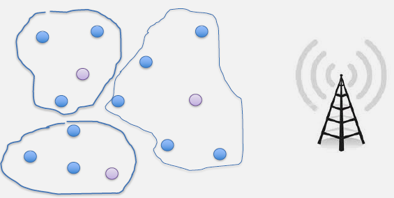
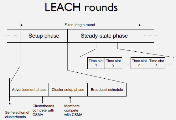
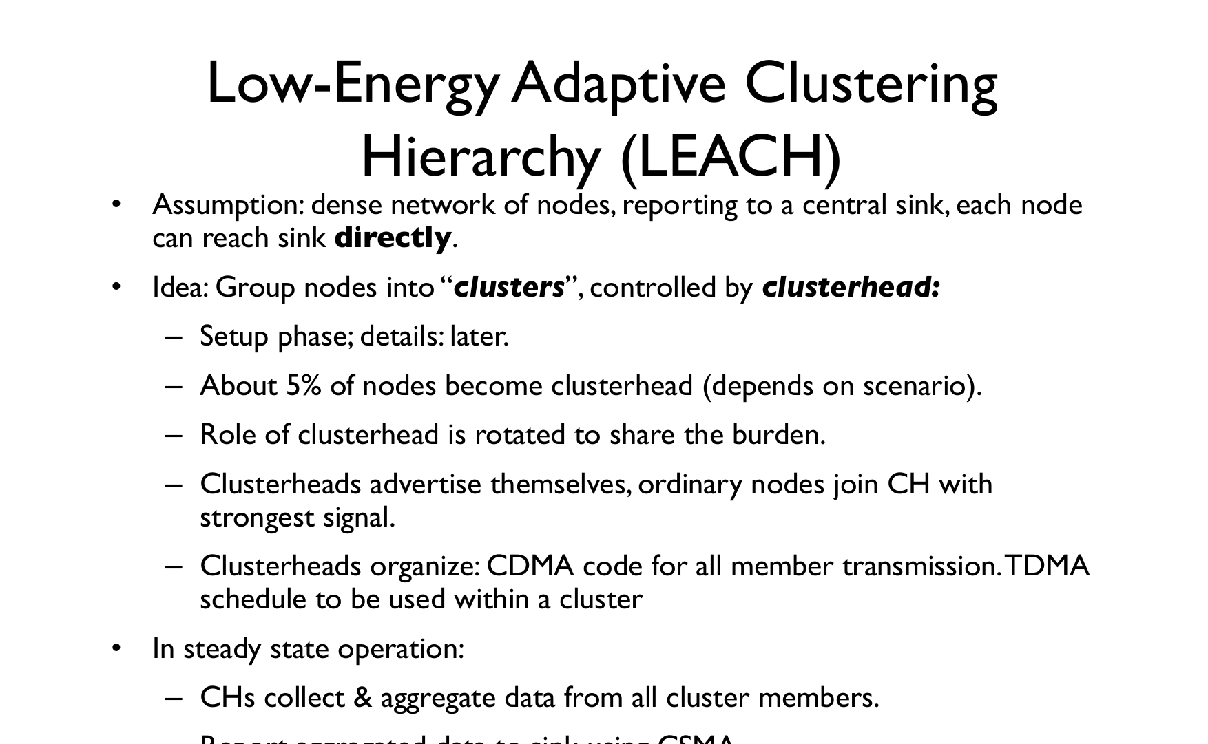
Examples: - LEACH (Low-Energy Adaptive Clustering Hierarchy): Randomized cluster head rotation - PEGASIS (Power-Efficient GAthering in Sensor Information Systems): Chain-based routing - TEEN (Threshold sensitive Energy Efficient sensor Network): Event-driven reporting - Geographic routing: Position-based forwarding
NoteAcademic Resource: Cambridge Mobile and Sensor Systems
Source: University of Cambridge, Mobile and Sensor Systems Course (Prof. Cecilia Mascolo)
370.4 Radio Duty Cycling
Radio duty cycling is one of the most effective energy conservation techniques in WSNs, reducing the time transceivers spend in energy-consuming states.
370.4.1 Duty Cycling Fundamentals
Duty Cycle Definition: The fraction of time a node’s radio is active (transmitting, receiving, or listening).
\[\text{Duty Cycle} = \frac{\text{Active Time}}{\text{Total Time}}\]
Example: A node awake 10ms every 100ms has a 10% duty cycle.
Impact: Reducing duty cycle from 100% to 1% can extend battery lifetime by 10-100x, depending on the relative power consumption of radio vs. other components.
NoteAcademic Resource: Dynamic Duty Cycling Strategies
Source: University of Cambridge - Mobile and Sensor Systems (Prof. Cecilia Mascolo)
370.4.2 Duty Cycling Approaches
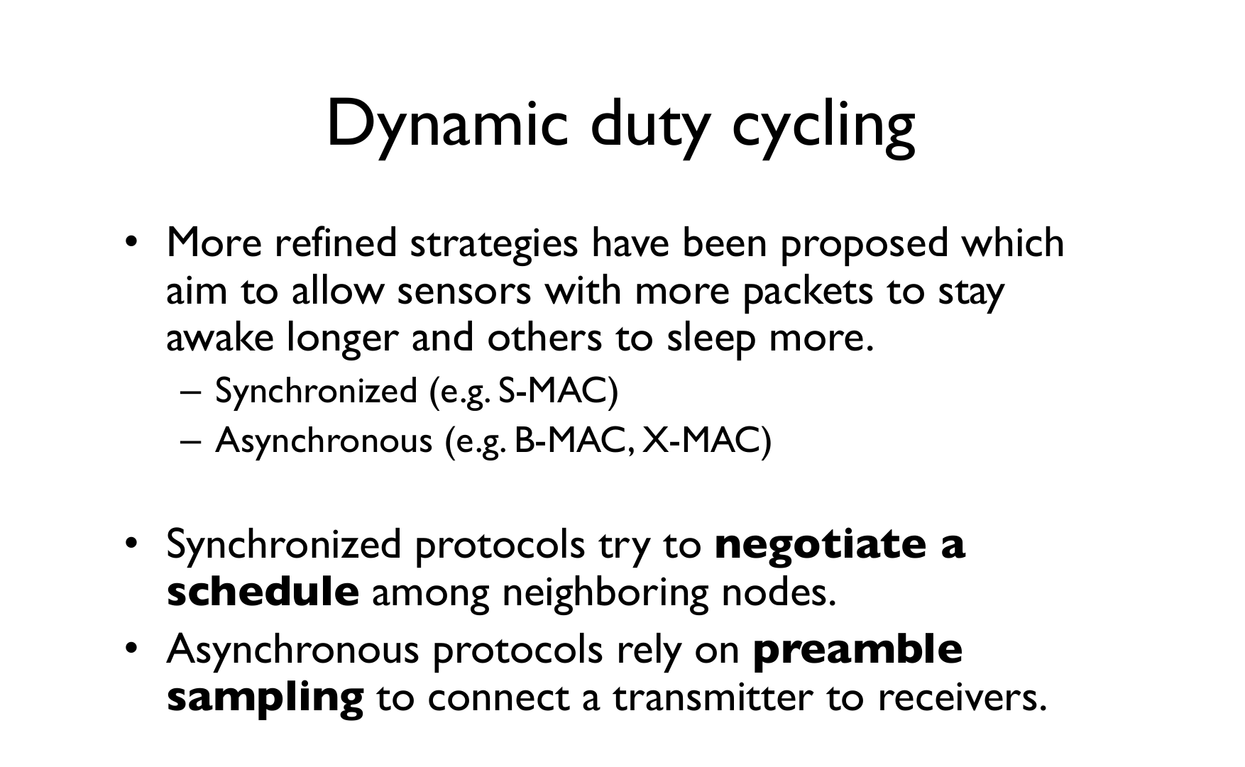
Synchronous Duty Cycling: Nodes coordinate wake/sleep schedules to ensure communication opportunities.
Characteristics: - Nodes wake up simultaneously - Requires clock synchronization - Lower latency for multi-hop communication - Examples: S-MAC, T-MAC
NoteAcademic Resource: S-MAC Protocol Architecture
Source: University of Cambridge - Mobile and Sensor Systems (Prof. Cecilia Mascolo)
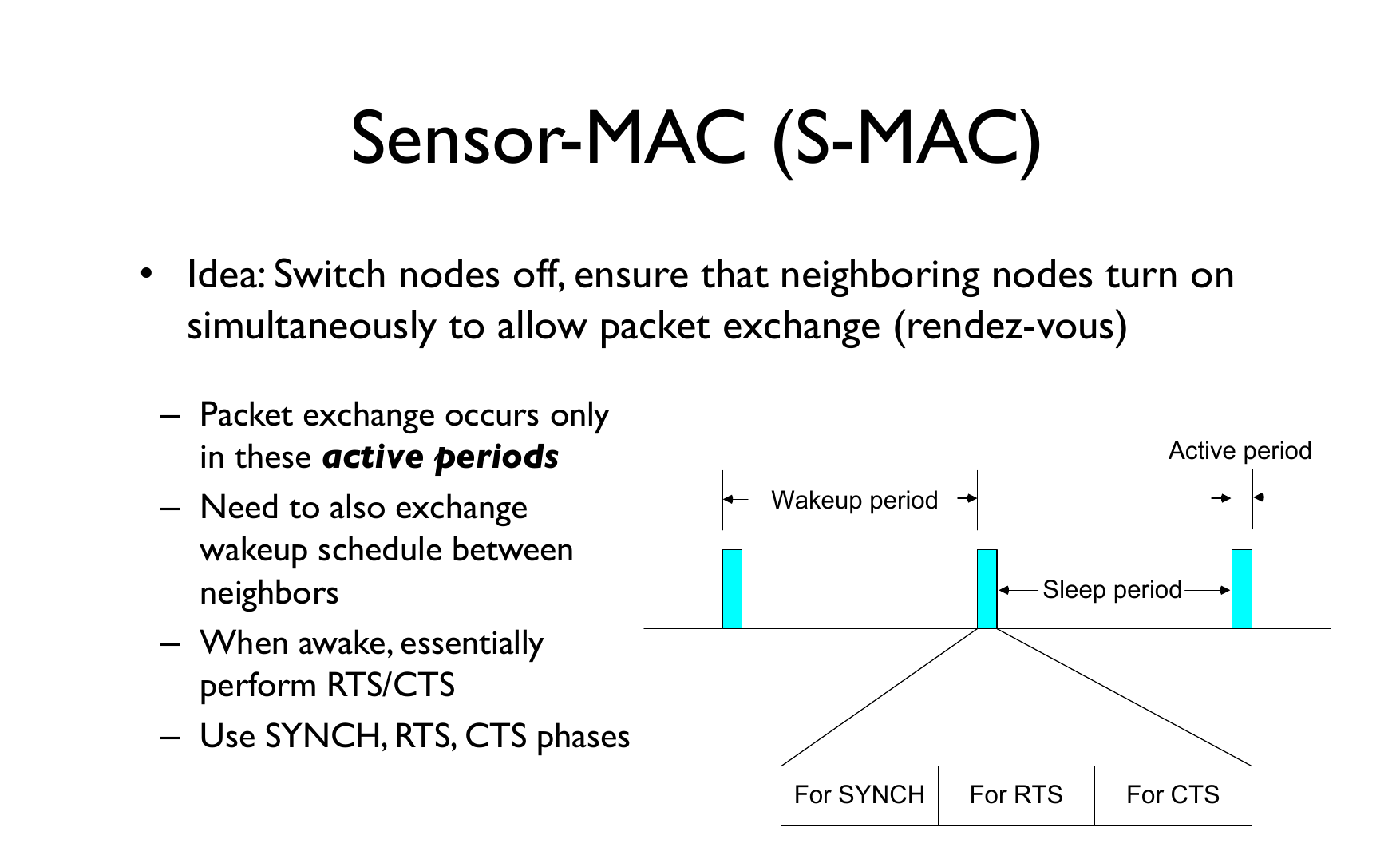
370.5 S-MAC Protocol: Visual Operation
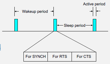
S-MAC (Sensor MAC) coordinates sleep schedules for energy efficiency.
370.5.1 The S-MAC Cycle
370.5.2 Step-by-Step Operation
%% fig-cap: "S-MAC step-by-step operation cycle"
%% fig-alt: "Flowchart showing S-MAC three-phase operation: synchronization with SYNC packets, listen period with RTS/CTS/DATA/ACK exchange, and sleep period with radio off"
%%{init: {'theme': 'base', 'themeVariables': {'primaryColor': '#2C3E50', 'primaryTextColor': '#fff', 'primaryBorderColor': '#1a252f', 'lineColor': '#16A085', 'secondaryColor': '#16A085', 'tertiaryColor': '#E67E22'}}}%%
flowchart TD
    subgraph sync["1. Synchronization"]
        S1["Nodes exchange SYNC packets"]
        S2["Agree on common schedule"]
    end

    subgraph listen["2. Listen Period"]
        L1["RTS: Request to Send"]
        L2["CTS: Clear to Send"]
        L3["DATA transmission"]
        L4["ACK receipt"]
    end

    subgraph sleep["3. Sleep Period"]
        Z1["Radio OFF"]
        Z2["Timer running"]
    end

    sync --> listen
    listen --> sleep
    sleep -->|"Timer expires"| sync

    style sync fill:#2C3E50,color:#fff
    style listen fill:#16A085,color:#fff
    style sleep fill:#7F8C8D,color:#fff
370.5.3 Energy Savings
| Duty Cycle | Listen Time | Sleep Time | Power Reduction |
|---|---|---|---|
| 100% | 100% | 0% | 0% (baseline) |
| 10% | 10% | 90% | ~90% |
| 1% | 1% | 99% | ~99% |
370.5.4 Key Insight
Nodes that hear the same SYNC adopt the same schedule, forming virtual clusters that can communicate efficiently.
Advantages: - Predictable communication windows - Efficient for scheduled traffic - Coordinated network operation
Challenges: - Synchronization overhead and drift - Global schedule may not suit all nodes - Less flexibility for event-driven traffic
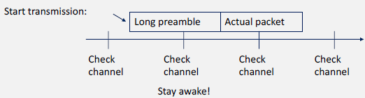
Asynchronous Duty Cycling: Nodes operate on independent schedules without global synchronization.
Characteristics: - No synchronization required - Senders must account for receiver schedules - Examples: B-MAC, X-MAC, RI-MAC
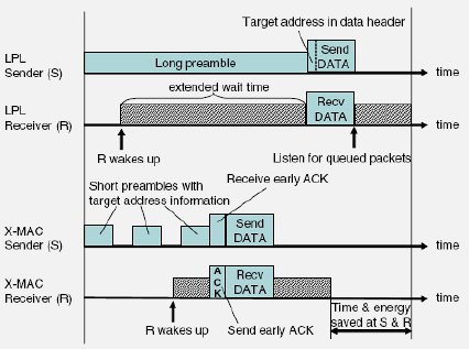
NoteAcademic Resource: X-MAC Short Preamble Protocol
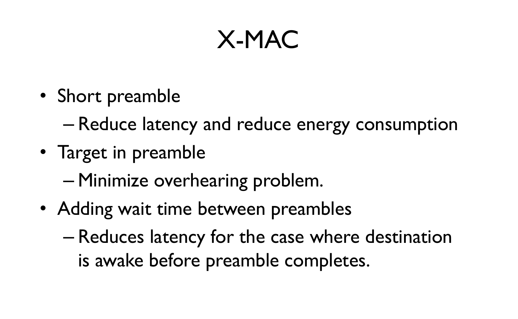
Source: University of Cambridge - Mobile and Sensor Systems (Prof. Cecilia Mascolo)
Mechanisms: - Preamble sampling: Sender transmits long preamble until receiver wakes - Wake-up beacons: Receivers announce availability - Receiver-initiated: Receivers poll for pending messages
Advantages: - No synchronization overhead - Flexible and adaptive - Supports mobile and heterogeneous networks
Challenges: - Potential latency increase - Energy cost of preambles or polling - Variable message delivery time
Hybrid Approaches: Combining synchronous and asynchronous techniques.
Examples: - Local synchronization within clusters, asynchronous between clusters - Schedule-based for regular traffic, on-demand for events - Adaptive switching based on traffic patterns
370.5.5 Advanced Duty Cycling Techniques
Adaptive Duty Cycling: Dynamically adjusting duty cycle based on conditions.
Parameters: - Traffic load (increase cycle during high activity) - Residual energy (reduce cycle when battery low) - Time of day (circadian patterns in environmental monitoring) - Event detection (increase sampling rate during events)
Predictive Duty Cycling: Using historical data and prediction models to optimize schedules.
Approaches: - Machine learning to predict traffic patterns - Correlation-based sensing (sensors with correlated readings coordinate) - Event prediction to pre-activate relevant nodes
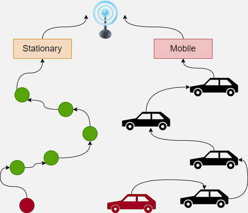
Hierarchical Duty Cycling: Different duty cycles for different node roles.
Structure: - Cluster heads: Higher duty cycle for availability - Regular nodes: Lower duty cycle for energy conservation - Gateway nodes: Always-on or high duty cycle
Wake-on-Radio: Special low-power radio listens continuously, waking main radio when messages arrive.
Characteristics: - Main radio sleeps indefinitely - Wake-up radio consumes micro-watts - Triggered wake-up for main radio - Ultra-low average power consumption
Technologies: - Dedicated wake-up receivers - Ultra-low-power always-on circuits - RF energy harvesting for wake-up
370.5.6 Performance Trade-offs
Energy vs. Latency: Lower duty cycles save energy but increase message delivery latency.
Mitigation: - Multi-hop forwarding during wake periods - Predictive wake-up for urgent messages - Adaptive cycles based on message priority
Energy vs. Reliability: Sleeping nodes may miss messages or events.
Solutions: - Redundant sensing coverage - Message retransmission mechanisms - Acknowledgment-based reliability - Wake-up on event detection
Energy vs. Throughput: Limited active time constrains data transmission capacity.
Balancing: - Efficient data aggregation and compression - Adaptive duty cycle during high-traffic periods - Buffering and batch transmission - Priority-based scheduling
370.6 Knowledge Check
Test your understanding of WSN fundamental concepts with these questions covering architecture, sensor nodes, and network topologies.
370.7 Summary
This chapter covered energy management and duty cycling in wireless sensor networks:
- Energy Consumption Profile: Radio communication dominates (50-300 mW), followed by processing (10-100 mW) and sensing (1-10 mW)
- Conservation Strategies: Duty cycling, data reduction, topology control, routing optimization, and energy harvesting
- Network Lifetime Metrics: FND (first node death), HND (half nodes dead), LND (last node death) for different application requirements
- Synchronous Duty Cycling: S-MAC coordinates sleep schedules through SYNC packets, enabling predictable communication windows
- Asynchronous Duty Cycling: B-MAC and X-MAC use preamble sampling, avoiding synchronization overhead but with variable latency
- Advanced Techniques: Adaptive, predictive, and hierarchical duty cycling; wake-on-radio for ultra-low power
- Trade-offs: Energy vs latency (sleeping increases delay), energy vs reliability (missed messages), energy vs throughput (limited active time)
370.8 What’s Next
Return to the WSN Overview: Fundamentals index page to review all chapters in this series, or continue to related topics:
- WSN Coverage Fundamentals - Coverage theory and deployment strategies
- WSN Tracking Fundamentals - Target localization algorithms
- Duty Cycling and Topology - Advanced MAC protocol details