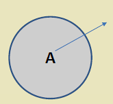
%% fig-alt: "Crossing-based coverage verification showing how checking finite crossing points (sensor boundary intersections) verifies coverage of infinite area points"
%%{init: {'theme': 'base', 'themeVariables': {'primaryColor': '#2C3E50', 'primaryTextColor': '#fff', 'primaryBorderColor': '#16A085', 'lineColor': '#16A085', 'secondaryColor': '#E67E22', 'tertiaryColor': '#ECF0F1', 'fontSize': '16px'}}}%%
graph TD
    subgraph "Crossing-Based Coverage Verification"
        REGION["Monitored<br/>Region A"]

        CROSS1["Crossing 1<br/>(S1 intersect S2)"]
        CROSS2["Crossing 2<br/>(S2 intersect S3)"]
        CROSS3["Crossing 3<br/>(S1 intersect boundary)"]
        CROSS4["Crossing 4<br/>(S3 intersect boundary)"]

        CHECK{"All crossings<br/>covered?"}

        COVERED["Complete<br/>Coverage"]
        GAPS["Coverage<br/>Holes"]
    end

    REGION --> CROSS1
    REGION --> CROSS2
    REGION --> CROSS3
    REGION --> CROSS4

    CROSS1 --> CHECK
    CROSS2 --> CHECK
    CROSS3 --> CHECK
    CROSS4 --> CHECK

    CHECK -->|"Yes"| COVERED
    CHECK -->|"No"| GAPS

    COVERED -.-> THEOREM["Zhang-Hou Theorem:<br/>Finite crossings<br/>verify infinite points"]
    GAPS -.-> REPAIR["Identify uncovered<br/>crossings for repair"]

    CHECK -.->|"Complexity:<br/>O(N squared) crossings<br/>vs infinite points"| EFFICIENT["Efficient<br/>verification"]

    style REGION fill:#2C3E50,stroke:#16A085,stroke-width:3px,color:#fff
    style CROSS1 fill:#E67E22,stroke:#2C3E50,stroke-width:2px,color:#fff
    style CROSS2 fill:#E67E22,stroke:#2C3E50,stroke-width:2px,color:#fff
    style CROSS3 fill:#E67E22,stroke:#2C3E50,stroke-width:2px,color:#fff
    style CROSS4 fill:#E67E22,stroke:#2C3E50,stroke-width:2px,color:#fff
    style CHECK fill:#3498DB,stroke:#2C3E50,stroke-width:3px,color:#fff
    style COVERED fill:#D5F4E6,stroke:#16A085,stroke-width:3px
    style GAPS fill:#FADBD8,stroke:#E74C3C,stroke-width:3px
    style THEOREM fill:#ECF0F1,stroke:#2C3E50,stroke-width:2px
    style REPAIR fill:#ECF0F1,stroke:#2C3E50,stroke-width:2px
    style EFFICIENT fill:#D5F4E6,stroke:#16A085,stroke-width:2px
364 WSN Coverage Algorithms
NoteKey Concepts
- Crossing Coverage Theory: Zhang-Hou theorem proving that checking finite crossing points verifies infinite area coverage
- OGDC Algorithm: Optimal Geographical Density Control - distributed algorithm achieving near-optimal triangular lattice coverage
- Virtual Force Algorithm: Coverage repair using simulated attractive/repulsive forces for mobile sensor repositioning
- Coverage Hole Detection: Identifying uncovered regions using Voronoi diagrams and crossing analysis
- Rotation Scheduling: Alternating active sensor sets to extend network lifetime while maintaining coverage
364.1 Learning Objectives
By the end of this chapter, you will be able to:
- Apply Crossing Theory: Use Zhang-Hou theorem to verify coverage with finite checks
- Implement OGDC: Design distributed coverage algorithms with optimal triangular lattice spacing
- Analyze Virtual Force: Understand how mobile sensors use simulated physics for coverage repair
- Design Rotation Schedules: Create energy-efficient coverage maintenance strategies
TipMVU: Minimum Viable Understanding
Core concept: Coverage verification reduces from checking infinite points to finite crossings using Zhang-Hou theorem. Why it matters: OGDC achieves 95%+ coverage with only 40-60% of sensors active, extending network lifetime 2-3x. Key takeaway: Optimal sensor spacing is sqrt(3) x Rs (triangular lattice) - memorize this for deployment planning.
364.2 Prerequisites
Before diving into this chapter, you should be familiar with:
- WSN Coverage Fundamentals: Coverage definitions and connectivity concepts
- WSN Coverage Types: Area, point, and barrier coverage problems
NoteRelated Chapters
Fundamentals: - WSN Coverage Fundamentals - Coverage basics and connectivity - WSN Coverage Types - Area, point, and barrier coverage
Implementations: - WSN Coverage Implementations - Hands-on labs and Python code
Review: - WSN Coverage Review - Comprehensive coverage quiz and summary
364.3 Coverage Maintenance Algorithms
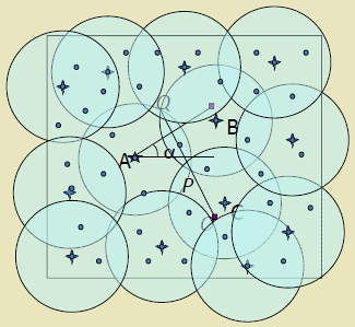
364.3.1 Crossing Coverage Theory
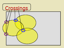
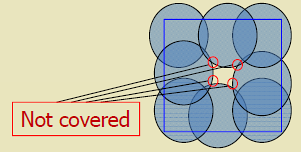
Theorem (Zhang and Hou):
A continuous region is completely covered if and only if: 1. There exist crossings in the region 2. Every crossing is covered
Definitions:
- Crossing:
- Intersection point between: - Two sensor coverage disk boundaries, OR - Monitored space boundary and a disk boundary
Why Crossings Matter:
If all crossings are covered, then all points are covered. This reduces the coverage verification problem from checking infinite points to checking finite crossings.
364.3.2 Optimal Geographical Density Control (OGDC)
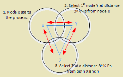
OGDC is a distributed, localized algorithm that achieves near-optimal coverage with minimal active sensors.
Key Idea:
Nodes self-organize into a triangular lattice pattern, which is provably near-optimal for disk coverage.
Optimal Spacing:
For sensors with sensing range Rs, optimal spacing between active sensors is:
\[ d_{optimal} = \sqrt{3} \cdot R_s \]
This minimizes overlap while maintaining complete coverage.
%% fig-alt: "OGDC triangular lattice formation showing optimal sqrt(3) x Rs spacing between active nodes for near-optimal coverage with minimal overlap"
%%{init: {'theme': 'base', 'themeVariables': {'primaryColor': '#2C3E50', 'primaryTextColor': '#fff', 'primaryBorderColor': '#16A085', 'lineColor': '#16A085', 'secondaryColor': '#E67E22', 'tertiaryColor': '#ECF0F1', 'fontSize': '16px'}}}%%
graph TD
    subgraph "OGDC Triangular Lattice Formation"
        START["Starting Node<br/>(Volunteer)"]

        N1["Node 1<br/>Distance: sqrt(3) x Rs"]
        N2["Node 2<br/>Distance: sqrt(3) x Rs"]
        N3["Node 3<br/>Distance: sqrt(3) x Rs"]
        N4["Node 4<br/>Distance: sqrt(3) x Rs"]
        N5["Node 5<br/>Distance: sqrt(3) x Rs"]
        N6["Node 6<br/>Distance: sqrt(3) x Rs"]

        SLEEP1["Sleeping nodes<br/>(Energy conservation)"]
    end

    START --> N1
    START --> N2
    START --> N3
    START --> N4
    START --> N5
    START --> N6

    N1 -.->|"sqrt(3) x Rs spacing"| N2
    N2 -.->|"sqrt(3) x Rs spacing"| N3
    N3 -.->|"sqrt(3) x Rs spacing"| N4
    N4 -.->|"sqrt(3) x Rs spacing"| N5
    N5 -.->|"sqrt(3) x Rs spacing"| N6
    N6 -.->|"sqrt(3) x Rs spacing"| N1

    START -.-> SLEEP1

    LATTICE["Triangular Lattice<br/>Near-optimal coverage<br/>Minimal overlap"]

    N3 --> LATTICE
    N4 --> LATTICE

    BENEFIT["Benefits:<br/>95% coverage<br/>40-60% nodes active<br/>2-2.5x lifetime"]

    LATTICE -.-> BENEFIT

    style START fill:#E67E22,stroke:#2C3E50,stroke-width:3px,color:#fff
    style N1 fill:#16A085,stroke:#2C3E50,stroke-width:3px,color:#fff
    style N2 fill:#16A085,stroke:#2C3E50,stroke-width:3px,color:#fff
    style N3 fill:#16A085,stroke:#2C3E50,stroke-width:3px,color:#fff
    style N4 fill:#16A085,stroke:#2C3E50,stroke-width:3px,color:#fff
    style N5 fill:#16A085,stroke:#2C3E50,stroke-width:3px,color:#fff
    style N6 fill:#16A085,stroke:#2C3E50,stroke-width:3px,color:#fff
    style SLEEP1 fill:#95A5A6,stroke:#2C3E50,stroke-width:2px,color:#fff
    style LATTICE fill:#3498DB,stroke:#2C3E50,stroke-width:3px,color:#fff
    style BENEFIT fill:#D5F4E6,stroke:#16A085,stroke-width:2px
364.3.3 OGDC Algorithm Phases
Phase 1: Starting Node Selection
def ogdc_select_starting_node(nodes, volunteer_probability=0.1):
    """
    Phase 1: Randomly select starting node using exponential backoff
    """
    for node in nodes:
        if random.random() < volunteer_probability:
            # Volunteer to be starting node
            backoff_time = random.uniform(0, MAX_BACKOFF)
            node.backoff_timer = backoff_time

    # Node with shortest backoff becomes starting node
    time.sleep(max(n.backoff_timer for n in nodes))

    # First node whose timer expires wins
    starting_node = min(nodes, key=lambda n: n.backoff_timer)

    starting_node.activate()
    starting_node.broadcast_start_message()

    return starting_node

class StartMessage:
    def __init__(self, sender_id, sender_position, preferred_direction):
        self.sender_id = sender_id
        self.position = sender_position
        self.direction = preferred_direction  # Random angle 0-360 degrees
Phase 2: Iterative Node Activation
364.3.4 OGDC Performance
Coverage Quality: - Achieves >95% coverage with ~60% of nodes - Near-optimal (within 5% of theoretical minimum)
Energy Efficiency: - 40-60% nodes sleep at any time - Network lifetime extends by 1.67-2.5x
Scalability: - Distributed: No central coordinator - Localized: Only neighbor communication - Scales to thousands of nodes
364.3.5 Virtual Force Algorithm
Virtual force algorithms (Zou and Chakrabarty, 2003) improve coverage through simulated physics:
Algorithm Components:
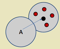
Repulsive forces: Sensors too close together (overlapping coverage) repel each other, spreading out to reduce redundancy. Force is proportional to 1/distance squared.
Attractive forces: Coverage holes exert attractive force on nearby sensors, pulling them toward uncovered regions.
Boundary forces: Virtual obstacles at deployment boundaries prevent sensors from moving outside target area.
Equilibrium: System iterates until forces balance, reaching stable configuration with improved coverage.
%% fig-alt: "Virtual force algorithm showing repulsive forces between nearby sensors and attractive forces from coverage holes"
%%{init: {'theme': 'base', 'themeVariables': {'primaryColor': '#2C3E50', 'primaryTextColor': '#fff', 'primaryBorderColor': '#16A085', 'lineColor': '#16A085', 'secondaryColor': '#E67E22', 'tertiaryColor': '#ECF0F1', 'fontSize': '16px'}}}%%
graph TD
    subgraph "Virtual Force Algorithm"
        S1["Sensor S1"]
        S2["Sensor S2<br/>(Too close)"]
        S3["Sensor S3"]

        HOLE["Coverage<br/>Hole"]

        BOUNDARY["Deployment<br/>Boundary"]
    end

    S1 <-->|"Repulsive<br/>Force"| S2
    S2 <-->|"Repulsive<br/>Force"| S3

    HOLE -.->|"Attractive<br/>Force"| S1
    HOLE -.->|"Attractive<br/>Force"| S3

    BOUNDARY -.->|"Boundary<br/>Force"| S1
    BOUNDARY -.->|"Boundary<br/>Force"| S3

    RESULT["Equilibrium:<br/>Sensors spread out<br/>Holes filled<br/>Stay in bounds"]

    S1 --> RESULT
    S2 --> RESULT
    S3 --> RESULT

    style S1 fill:#16A085,stroke:#2C3E50,stroke-width:3px,color:#fff
    style S2 fill:#16A085,stroke:#2C3E50,stroke-width:3px,color:#fff
    style S3 fill:#16A085,stroke:#2C3E50,stroke-width:3px,color:#fff
    style HOLE fill:#E74C3C,stroke:#2C3E50,stroke-width:3px,color:#fff
    style BOUNDARY fill:#7F8C8D,stroke:#2C3E50,stroke-width:2px,color:#fff
    style RESULT fill:#D5F4E6,stroke:#16A085,stroke-width:2px
Algorithm Steps:
For each sensor: 1. Calculate forces from all neighbors (repulsive) and coverage holes (attractive) 2. Compute net force vector 3. Move sensor incrementally in force direction 4. Repeat until convergence (forces below threshold)
Requirements: Mobile sensors with locomotion capability (wheeled robots, aerial drones). Not applicable to static sensors.
Performance: Improves random deployment coverage from 75% to 95% through iterative repositioning.
Costs: - Mobility hardware: Expensive and energy-intensive - Localization: Sensors must know their positions (GPS, trilateration) - Computation: Force calculations require neighbor positions
Applications: Underwater sensor networks (AUVs can relocate), aerial drone swarms, disaster response robots. Not practical for scattered static sensors.
Alternative for static networks: Use virtual forces to plan initial deployment, then execute with static sensors.
364.4 Algorithm Comparison
| Algorithm | Type | Coverage | Active Sensors | Complexity | Best For |
|---|---|---|---|---|---|
| Crossing Theory | Verification | 100% verified | N/A | O(N squared) | Coverage checking |
| OGDC | Activation | 95-98% | 40-60% | O(N log N) | Static WSN |
| Virtual Force | Repositioning | 90-95% | 100% | O(N squared) | Mobile sensors |
| Grid Deployment | Placement | 100% | 100% | O(1) | Accessible terrain |
364.5 Summary
This chapter covered three key coverage algorithms:
Key Takeaways:
Crossing Theory - Zhang-Hou theorem enables efficient coverage verification by checking O(N squared) crossing points instead of infinite area points.
OGDC Algorithm - Distributed, localized algorithm achieving near-optimal triangular lattice (sqrt(3) x Rs spacing) with 40-60% energy savings.
Virtual Force - Mobile sensor repositioning using simulated physics (repulsive between sensors, attractive toward holes). Best for drone swarms and disaster response.
Algorithm Selection - Use crossing theory for verification, OGDC for static WSN activation, virtual force for mobile sensor coverage repair.
364.6 What’s Next?
Now that you understand coverage algorithms, the next chapter provides hands-on labs and Python implementations.
Continue to WSN Coverage Implementations - Build and test coverage systems with practical labs and code examples.