Time: ~15 min | Level: Intermediate | Unit: P03.C03.U10
126.2 Learning Objectives
By the end of this section, you will be able to:
Understand precision agriculture IoT systems and their ROI drivers
Design livestock monitoring solutions with sensor fusion
Calculate irrigation optimization benefits using worked examples
Apply greenhouse climate control for yield improvement
Analyze multi-sensor data fusion for crop yield prediction
NoteVideo: Digital Agriculture and Connected Farming
Explore how IoT sensors optimize crop yields through precision agriculture.
NoteVideo: Connected Livestock Management
See how livestock tracking improves animal health monitoring and herd management.
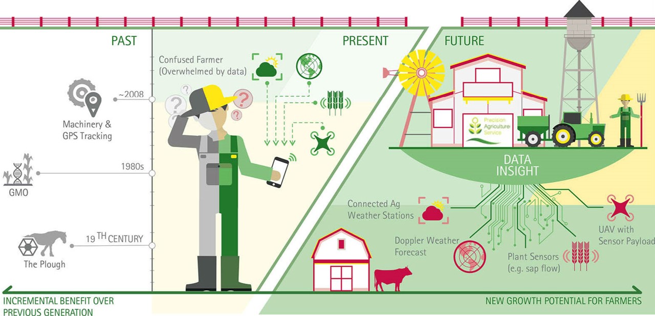
126.3 Precision Agriculture Overview
Precision Agriculture
Figure 126.1: Precision agriculture teams pair soil sensors with drone imagery to fine-tune irrigation and optimize crop yields.
Key Technologies:
Technology
Application
Benefit
Soil sensors
Moisture, nutrients, pH
Precise irrigation and fertilization
Weather stations
Microclimate monitoring
Disease prediction, frost alerts
Drones
Multispectral imaging
Early stress detection
GPS guidance
Variable rate application
Reduced input waste
Satellite imagery
Field-scale monitoring
Coverage assessment
126.4 Connected Livestock: 1.4 Billion Cattle
TipThe Connected Livestock Opportunity
Scale of the Problem:
With approximately 1.4 billion cattle worldwide, livestock represents one of the largest IoT deployment opportunities in agriculture. The challenge: animals can’t tell you when they first get sick.
The Early Detection Problem:
Challenge
Traditional Approach
IoT Solution
Illness detection
Wait for visible symptoms
Continuous monitoring detects subtle changes
Heat detection (breeding)
Manual observation (21-day cycles)
Activity sensors detect estrus behavior
Calving alerts
Night checks every 2-3 hours
Temperature/activity sensors predict labor
Feed efficiency
Herd-level estimates
Individual intake monitoring
Grazing patterns
Assume uniform grazing
GPS tracks overgrazing, underused areas
Key Insight: IoT sensors cannot diagnose an illness, but they alert farmers when something needs attention - shifting from reactive to proactive herd management.
Sensor Technologies for Livestock:
Sensor Type
What It Measures
Early Warning For
Bolus (rumen)
Core body temperature, pH
Fever, acidosis, heat stress
Collar/ear tag
Activity, rumination time
Lameness, illness, estrus
GPS tracker
Location, movement patterns
Predators, fence breaches, sick animals
Weight scale (walkover)
Daily weight changes
Growth rate, illness onset
Methane sensor
Emissions per animal
Feed efficiency, breeding selection
Economic Impact: - Early illness detection: $300-500 saved per prevented severe case - Heat detection accuracy: 80% to 95% (reduce missed breeding cycles) - Calving intervention timing: Reduce calf mortality by 30-50% - Feed optimization: 10-15% reduction in feed costs
Connected Livestock in Field
Figure 126.2: Livestock collars transmit health and location data, enabling early intervention when herd patterns change.
Livestock Management Dashboard
Figure 126.3: Digital twin dashboards blend satellite imagery and IoT telemetry to track herd movement and pasture conditions.
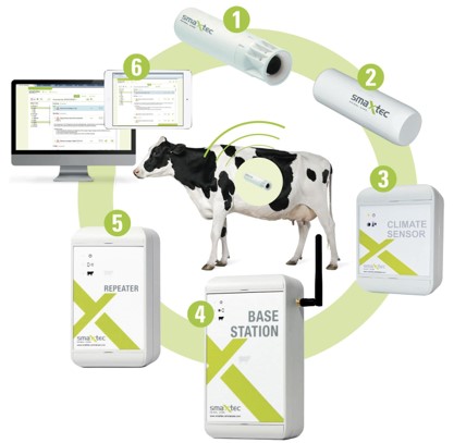
126.5 Case Study: Rumen Bolus System Architecture
The smaXtec system exemplifies modern livestock IoT with an ingestible sensor that lives in the cow’s rumen for its entire productive life:
Flowchart diagram
Figure 126.4: Rumen bolus livestock monitoring system: Ingestible sensor in cow’s rumen transmits temperature, pH, and activity data via low-power radio to barn gateway, cloud analytics detects health anomalies and heat events, mobile app alerts farmer with actionable recommendations.
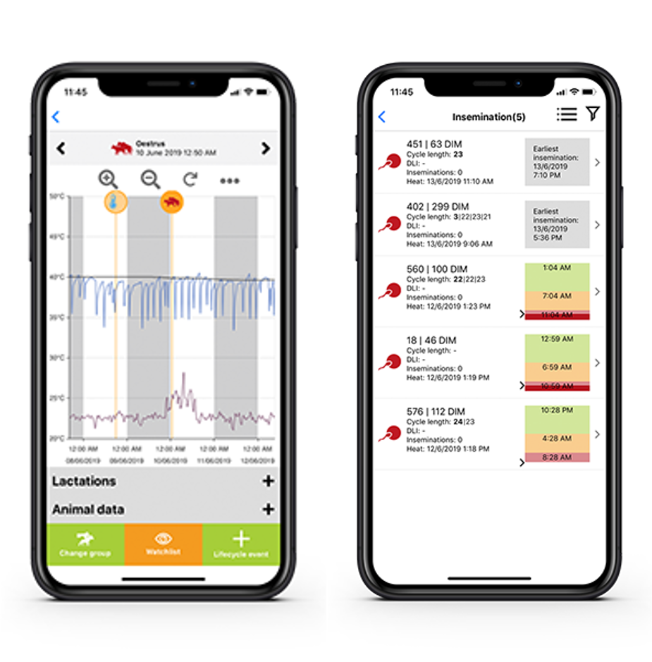
What the Bolus Detects (continuous monitoring from inside the cow):
Measurement
Detection Capability
Time Advantage
pH level
Fermentation disorders (acidosis)
24-48 hours before visible symptoms
Activity
Estrus (heat), onset of illness
Auto-detect 21-day breeding window
Temperature
Fever, metabolic disorders, calving
Predict calving within 6-12 hours
Drinking behavior
Hydration, heat stress
Detect before dehydration
Alert Examples (from smaXtec mobile app): - “Cow #46: Temperature increase - Health alert” - “Cow #23: Temperature drop - Likely calving within 12 hours” - “Cow #89: Less drinking cycles - Check water access”
126.6 Worked Example: Center Pivot Irrigation Optimization
Scenario: A Kansas wheat farmer is upgrading a 130-acre center pivot irrigation system with IoT-enabled variable rate irrigation (VRI) to address yield variability caused by soil type differences across the circular field.
Given: - Field area: 130 acres under center pivot (circular) - Pivot radius: 400 meters (1,312 feet) - Soil zones: 4 distinct zones from soil electrical conductivity (EC) mapping - Zone A (32 acres): Sandy loam, high infiltration, 15% of pivot - Zone B (45 acres): Loam, moderate infiltration, 35% of pivot - Zone C (38 acres): Clay loam, low infiltration, 29% of pivot - Zone D (15 acres): Heavy clay, very low infiltration, 21% of pivot - Water source capacity: 800 GPM (gallons per minute) - Electricity cost: $0.08/kWh - Previous season uniform application: 18 inches total, $14,500 water/energy cost - Yield variation: 35-65 bushels/acre (high variability)
Steps:
Install IoT sensor network: Deploy 12 soil moisture sensors across 4 zones (3 per zone) at 12-inch depth connected via LoRaWAN to field edge gateway.
Sensor cost: 12 x $350 = $4,200
Gateway + installation: $1,800
Total infrastructure: $6,000
Calculate zone-specific water requirements (based on soil water holding capacity):
Zone A (sandy): Needs 22 inches (low retention, frequent light irrigation)
Zone B (loam): Needs 16 inches (optimal, baseline)
Zone C (clay loam): Needs 14 inches (holds water longer)
Zone D (heavy clay): Needs 12 inches (risk of waterlogging)
Configure VRI prescription map: Program pivot controller with GPS-triggered nozzle adjustments.
Zone A: 122% of base rate (more frequent, lighter passes)
Zone B: 100% base rate
Zone C: 87% of base rate
Zone D: 75% of base rate
Calculate water and energy savings:
Previous total: 18 in x 130 acres = 2,340 acre-inches
Water reduction: (2,340 - 2,136) / 2,340 = 8.7% reduction
Energy savings: 8.7% x $14,500 = $1,262/year
Project yield improvement: Eliminating waterlogging in Zone D and drought stress in Zone A.
Zone A yield increase: 45 to 55 bu/acre (+10 bu x 32 acres = 320 bu)
Zone D yield increase: 35 to 50 bu/acre (+15 bu x 15 acres = 225 bu)
Total additional yield: 545 bushels x $6/bu = $3,270/year
Result: VRI system payback period of 1.3 years. Annual benefits: - Water savings: 204 acre-inches (8.7% reduction) - Energy savings: $1,262/year - Yield improvement: $3,270/year (545 additional bushels) - Total annual benefit: $4,532 on $6,000 investment
Key Insight: Variable rate irrigation ROI comes primarily from yield improvement in problem zones, not water savings. The 8.7% water reduction alone would not justify the investment; the yield gains from eliminating over/under-watering in extreme soil zones provide the economic driver.
126.7 Worked Example: Greenhouse Climate Control
Scenario: A Dutch greenhouse operator is optimizing a 2-hectare tomato greenhouse to maximize yield while minimizing natural gas consumption for heating.
Given: - Greenhouse area: 20,000 m2 (2 hectares) - Crop: Indeterminate tomatoes (year-round production) - Current yield: 55 kg/m2/year (industry average for Netherlands) - Target yield: 70 kg/m2/year (top-tier performance) - Natural gas price: EUR 0.80/m3 - Current annual gas consumption: 45 m3/m2 = 900,000 m3 total - Electricity cost: EUR 0.15/kWh - Tomato price: EUR 1.20/kg average
Steps:
Deploy IoT sensor network (per 500 m2 zone = 40 zones total):
Temperature/humidity sensors: 80 (2 per zone at crop and roof level)
CO2 sensors: 40 (1 per zone)
PAR light sensors: 20 (every 1,000 m2)
Substrate moisture/EC sensors: 160 (4 per zone in growing medium)
Total sensors: 300
Cost: EUR 45,000 (sensors + wiring + integration)
Establish optimal setpoints by growth stage:
Parameter
Vegetative
Flowering
Fruiting
Day temp
21-23C
20-22C
19-21C
Night temp
17-18C
16-17C
15-16C
Humidity
70-80%
65-75%
60-70%
CO2
800 ppm
1000 ppm
900 ppm
PAR target
400 umol
500 umol
450 umol
Implement predictive heating control: Use weather forecast integration to pre-heat greenhouse before cold nights rather than reactive heating.
Prediction horizon: 6 hours
Energy model accuracy: +/-5% of actual consumption
Buffer capacity: Thermal mass in concrete floor + water pipes
Calculate energy savings from optimization:
Temperature integration (average 24h temp vs. fixed setpoints): -12% gas
Predictive vs. reactive heating: -8% gas
Screen management optimization: -5% gas
Total gas reduction: 25% x 900,000 m3 = 225,000 m3 saved
Cost savings: 225,000 x EUR 0.80 = EUR 180,000/year
Project yield improvement from precise climate control:
Reduced temperature stress: +8% yield
Optimal CO2 enrichment timing: +6% yield
Disease reduction from humidity control: +4% yield
Compound improvement: 55 x 1.18 = 65 kg/m2 (conservative)
Additional yield: (65-55) x 20,000 m2 x EUR 1.20 = EUR 240,000/year
Result: Total annual benefit of EUR 420,000 on EUR 45,000 sensor investment (9.3x ROI in year one). Payback period: 39 days of operation.
Energy cost reduction: EUR 180,000/year (25% gas savings)
Additional benefits: Reduced labor for manual monitoring, disease early warning
Key Insight: Greenhouse IoT delivers compounding returns because energy optimization and yield improvement are synergistic. Precise temperature control simultaneously reduces heating costs AND improves plant growth. The sensor density (1 per 67 m2) seems high but is justified by the EUR 2,100/m2 annual revenue in intensive greenhouse production.
126.8 Worked Example: Crop Yield Prediction
Scenario: A California almond grower is building a yield prediction model by fusing data from soil sensors, weather stations, satellite imagery, and historical harvest records across a 2,000-acre orchard to forecast tonnage 6 weeks before harvest.
Given: - Orchard size: 2,000 acres (809 hectares) of mature Nonpareil almonds - Tree density: 110 trees per acre (220,000 trees total) - Average yield: 2,400 lbs/acre (2,400 tons total crop) - Almond price volatility: $2.00-$4.50 per pound - Current yield uncertainty: +/- 25% until 2 weeks pre-harvest - Harvest labor cost: $180/acre (contracted 60 days ahead) - Processing plant scheduling: Committed 45 days ahead - Sensor infrastructure: 40 soil moisture sensors, 4 weather stations
Steps:
Identify predictive variables and data sources:
Variable
Data Source
Correlation to Yield
Update Frequency
Bloom temperature
Weather stations
r = 0.72
Historical (Feb)
Chill hours
Weather stations
r = 0.68
Season total
April soil moisture
Capacitive sensors
r = 0.61
Daily
NDVI at hull split
Sentinel-2 satellite
r = 0.78
5-day revisit
Nut load (visual)
Drone sampling
r = 0.85
Bi-weekly
Historical trend
Harvest records
r = 0.55
Annual
Deploy additional sensing for model inputs:
Automated weather stations: 4 units across microclimates ($12,000 total)
Drone + RGB/multispectral: $8,500 (existing, reallocate for nut counting)
Value: 2,400 tons x 2,000 lbs x 2% x $3/lb = $288,000
Marketing timing:
Hedge forward contracts with confidence: +$0.05/lb average
Value: 4.8M lbs x $0.05 = $240,000
Model accuracy validation:
Year 1: Prediction within 4% at T-45 (vs. 18% baseline)
Year 2: Prediction within 3% at T-45 (model refined)
Target: <5% error at commitment point
Result: Yield prediction system delivers annual value of $564,000: - Labor optimization: $36,000 - Harvest timing improvement: $288,000 - Marketing advantage: $240,000 - System annual cost: $28,900 - Net benefit: $535,100 - ROI: 1,852%
Key Insight: In tree crops like almonds, yield prediction value comes from matching harvest infrastructure to actual crop volume. A 20% over-estimate means contracting 400 excess labor days at $180 each; a 20% under-estimate means almonds on the ground losing value. Multi-sensor fusion achieves prediction accuracy impossible from any single data source because yield integrates weather, soil, and tree health factors across the entire growing season.
126.9 Worked Example: Poultry House Feed Conversion
Scenario: An Arkansas broiler producer is deploying IoT environmental monitoring to improve feed conversion ratio (FCR) across 16 poultry houses, targeting a 0.05-point FCR reduction worth millions in feed savings.
Given: - Number of houses: 16 (40,000 birds each = 640,000 birds per flock) - Flocks per year: 6.5 (50-day cycle + 10-day cleanout) - Annual bird placements: 4.16 million birds - Target market weight: 6.5 lbs live weight - Current FCR: 1.78 (lbs feed per lb live gain) - Feed cost: $0.18 per pound - Bird value: $0.58 per pound live weight - Mortality rate: 4.2% - Major FCR factors: Temperature, ventilation, ammonia, litter moisture
Steps:
Deploy environmental sensor network per house:
Temperature sensors: 12 per house (3 zones x 4 heights) = 192 total
Humidity sensors: 4 per house = 64 total
Ammonia sensors: 2 per house = 32 total
CO2 sensors: 2 per house = 32 total
Water/feed consumption meters: 2 per house = 32 total
Total sensors: 352
Cost per house: $4,500 (sensors + controller integration)
Total infrastructure: $72,000
Establish FCR impact relationships:
Environmental Factor
Optimal Range
FCR Impact (per unit deviation)
Temperature (F)
70-82 (age-adjusted)
+0.01 FCR per 2F deviation
Ammonia (ppm)
<25 ppm
+0.02 FCR per 10 ppm above
CO2 (ppm)
<3,000 ppm
+0.01 FCR per 1,000 ppm above
Litter moisture (%)
20-30%
+0.015 FCR per 5% deviation
Light uniformity
>90%
+0.01 FCR if <85%
Calculate current environmental deviations:
Average temperature deviation: 3F (poor air mixing in 8 of 16 houses)
Ammonia spikes: 35 ppm average in weeks 5-7 (ventilation timing)
Result: Poultry house IoT system delivers annual benefits of $265,800: - Feed savings from FCR improvement: $180,000 - Reduced mortality value: $62,800 - Energy optimization: $15,000 - Labor savings: $8,000 - System cost: $72,000 installation + $12,000/year maintenance - First-year ROI: ($265,800 - $84,000) / $72,000 = 252% - Payback period: 4.3 months
Key Insight: In poultry production, a 0.01-point FCR improvement is worth approximately $45,000 annually on a 4-million-bird operation. Environmental monitoring enables precise ventilation control that simultaneously improves FCR, reduces mortality, and lowers energy costs. The key is sensor density sufficient to detect microclimates within houses - temperature can vary 8-10F from floor to ceiling and end to end, and birds at floor level experience conditions invisible to a single ceiling-mounted sensor.
126.10 Knowledge Check
Show code
{const container =document.getElementById('kc-usecase-agriculture');if (container &&typeof InlineKnowledgeCheck !=='undefined') { container.innerHTML=''; container.appendChild(InlineKnowledgeCheck.create({question:"A 500-hectare farm is deploying IoT soil moisture sensors to optimize irrigation. Water costs $800/hectare annually, and overwatering wastes 30% while underwatering reduces yield by 25% ($2,000/hectare crop value). Sensors cost $150 each with 10-hectare coverage (50 sensors needed) plus $20/month connectivity per sensor. What is the approximate annual ROI?",options: [ {text:"50-75% - modest improvement in irrigation efficiency",correct:false,feedback:"The calculation shows much higher returns. Water savings alone: 500 ha x $800 x 30% waste eliminated = $120,000. Yield protection: potential $250,000 value. Combined benefit far exceeds the ~$13,500 annual sensor cost."}, {text:"200-400% - good ROI typical for agricultural IoT",correct:false,feedback:"Agricultural IoT often delivers even higher returns when both input costs (water, fertilizer) and yield protection are considered. The combined benefit in this scenario exceeds 1,000% ROI."}, {text:"Over 1,000% - precision irrigation delivers exceptional returns",correct:true,feedback:"Correct! Annual sensor cost: 50 x $150/5 years + 50 x $20 x 12 = $13,500. Water savings: $120,000 (30% of $400,000 water budget). Yield protection: ~$125,000 (avoiding underwatering losses on affected hectares). Total benefit: $245,000 / $13,500 = 1,815% ROI. Precision agriculture is one of the highest-ROI IoT applications."}, {text:"Negative - sensor costs exceed water savings",correct:false,feedback:"Sensor costs ($13,500/year) are a tiny fraction of potential savings ($245,000). Even water savings alone ($120,000) deliver 8x return on sensor investment."} ],difficulty:"hard",topic:"iot-use-cases-agriculture" })); }}