%% fig-alt: "Radar chart style comparison of three tracking formulations across five dimensions: Push-based scores high on real-time capability and tracking accuracy but low on energy efficiency and scalability. Poll-based scores high on energy efficiency and scalability but low on real-time capability. Guided scores high on interception capability and accuracy but requires mobile infrastructure."
%%{init: {'theme': 'base', 'themeVariables': { 'primaryColor': '#2C3E50', 'primaryTextColor': '#fff', 'primaryBorderColor': '#16A085', 'lineColor': '#16A085', 'secondaryColor': '#E67E22', 'tertiaryColor': '#7F8C8D'}}}%%
flowchart TB
    subgraph Push["PUSH-BASED"]
        P1["Real-time: HIGH"]
        P2["Energy: LOW"]
        P3["Scalability: MEDIUM"]
        P4["Best for: Wildlife monitoring<br/>Continuous surveillance"]
    end

    subgraph Poll["POLL-BASED"]
        Q1["Real-time: LOW"]
        Q2["Energy: HIGH"]
        Q3["Scalability: HIGH"]
        Q4["Best for: Asset tracking<br/>Inventory management"]
    end

    subgraph Guided["GUIDED"]
        G1["Real-time: HIGH"]
        G2["Energy: MEDIUM"]
        G3["Scalability: LOW"]
        G4["Best for: Intruder interception<br/>Search and rescue"]
    end

    Decision["Application<br/>Requirements"]

    Decision -->|"Need real-time +<br/>no mobile tracker"| Push
    Decision -->|"Battery critical +<br/>tolerate delay"| Poll
    Decision -->|"Must intercept +<br/>have drone/robot"| Guided

    style Push fill:#E67E22,stroke:#2C3E50,color:#fff
    style Poll fill:#16A085,stroke:#2C3E50,color:#fff
    style Guided fill:#2C3E50,stroke:#16A085,color:#fff
    style Decision fill:#7F8C8D,stroke:#2C3E50,color:#fff
394 WSN Tracking: Problem Formulations
394.1 Learning Objectives
By the end of this chapter, you will be able to:
- Understand Push-Based Tracking: Explain proactive sensor reporting for real-time tracking applications
- Understand Poll-Based Tracking: Design on-demand query systems for energy-efficient tracking
- Understand Guided Tracking: Implement active tracker interception using network-provided position updates
- Compare Formulations: Select the appropriate tracking formulation based on application requirements
- Analyze Trade-offs: Evaluate energy consumption vs latency trade-offs in tracking system design
TipMVU: Minimum Viable Understanding
Core concept: Three fundamental approaches exist for WSN tracking - push (sensors report proactively), poll (sink queries on-demand), and guided (active tracker intercepts target). Why it matters: Choosing the wrong formulation can waste 10x more energy or miss critical tracking events entirely. Key takeaway: Push for real-time critical applications, poll for battery-constrained large deployments, guided when physical interception is the goal.
394.2 Prerequisites
Before diving into this chapter, you should be familiar with:
- WSN Tracking: Fundamentals: Overview of tracking concepts and challenges
- Wireless Sensor Networks: Understanding WSN architecture, multi-hop communication, and coverage concepts
- WSN Overview: Fundamentals: Knowledge of sensor node capabilities and energy constraints
394.3 Target Tracking Problem Formulations
![]()
![]()
Detection Complexity Scenarios:
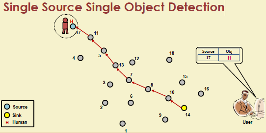
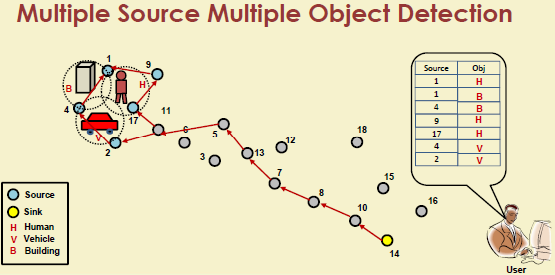
Target tracking algorithms estimate trajectories of one or more moving objects using distributed sensor measurements. The problem formulation determines how the algorithm operates and what trade-offs it makes.
394.3.1 Three Tracking Formulations

NoteAlternative View: Tracking Formulation Trade-offs
This variant presents the same three formulations through a trade-off comparison lens, helping system designers choose based on application requirements.
Selection Guidance: Choose Push for critical real-time applications (security, wildlife), Poll for large-scale deployments with battery constraints (smart cities), and Guided when physical interception is the goal (border security, rescue operations).
%% fig-alt: "Timeline showing target handoff sequence as target moves through WSN: at t=0 Sensor A detects target and becomes tracker, at t=2s Sensor A predicts target heading toward Sensor B and sends wake-up signal, at t=3s Sensor B wakes and confirms ready, at t=4s target enters overlap zone covered by both A and B, at t=5s Sensor B takes over as primary tracker and Sensor A returns to sleep - showing smooth handoff without tracking loss"
%%{init: {'theme': 'base', 'themeVariables': {'primaryColor': '#2C3E50', 'primaryTextColor': '#fff', 'primaryBorderColor': '#16A085', 'lineColor': '#E67E22', 'secondaryColor': '#16A085', 'tertiaryColor': '#E67E22', 'fontSize': '11px'}}}%%
sequenceDiagram
    participant T as Target
    participant A as Sensor A<br/>(Current Tracker)
    participant B as Sensor B<br/>(Next in Path)
    participant Sink as Base Station

    Note over T,Sink: HANDOFF SEQUENCE

    rect rgb(44, 62, 80)
    Note over A: t=0s: A is tracking
    T->>A: Detected at (10,5)
    A->>Sink: Position: (10,5)
    end

    rect rgb(22, 160, 133)
    Note over A: t=2s: Predict trajectory
    A->>A: Target heading East<br/>→ B is next
    A->>B: WAKE-UP signal<br/>(prepare for handoff)
    B->>B: Wake from sleep
    B->>A: READY ACK
    end

    rect rgb(230, 126, 34)
    Note over A,B: t=4s: Overlap zone
    T->>A: Still visible (12,5)
    T->>B: Now visible (12,5)
    A->>Sink: Joint estimate
    B->>Sink: Joint estimate
    Note over Sink: Data fusion<br/>improves accuracy
    end

    rect rgb(44, 62, 80)
    Note over B: t=5s: Handoff complete
    B->>Sink: I am now primary
    A->>A: Return to sleep
    T->>B: Tracking continues
    end

    Note over T,Sink: Zero tracking loss!
394.3.2 Push-Based Formulation
Concept: Sensors proactively collaborate to fuse data and periodically send reports toward the sink.

Example Application: Wildlife Tracking in Conservation Area
// Push-based animal tracking in wildlife reserve
#include <Arduino.h>
#include <LoRa.h>

const int PIR_SENSOR_PIN = 14;
const int REPORT_INTERVAL = 5000;  // 5 seconds (high frequency)
const int CLUSTER_HEAD_ID = 0;

struct TargetReport {
    uint8_t sensor_id;
    int16_t rssi;
    float temperature;  // Animal body heat signature
    uint32_t timestamp;
    float estimated_x, estimated_y;
};

bool isClusterHead = false;
std::vector<TargetReport> pending_reports;

void setup() {
    Serial.begin(115200);
    pinMode(PIR_SENSOR_PIN, INPUT);

    if (!LoRa.begin(915E6)) {
        Serial.println("LoRa init failed");
        while (1);
    }

    // Determine if this node is cluster head (ID-based or election)
    isClusterHead = (getNodeID() == CLUSTER_HEAD_ID);

    Serial.printf("Push-based tracker node %d initialized\n", getNodeID());
}

void loop() {
    // 1. Detect target
    if (detectTarget()) {
        Serial.println("Target detected!");

        // 2. Measure and report
        TargetReport report = measureTarget();

        if (isClusterHead) {
            // Cluster head: aggregate and forward to sink
            pending_reports.push_back(report);
            processReportsAndSend();
        } else {
            // Regular node: send to cluster head
            sendToClusterHead(report);
        }
    }

    delay(REPORT_INTERVAL);  // Periodic reporting
}

bool detectTarget() {
    // PIR sensor detects motion
    return digitalRead(PIR_SENSOR_PIN) == HIGH;
}

TargetReport measureTarget() {
    TargetReport report;
    report.sensor_id = getNodeID();
    report.rssi = LoRa.packetRssi();  // Signal strength
    report.temperature = readTemperature();  // Body heat
    report.timestamp = millis();

    // Local position estimate (trilateration in cluster head)
    report.estimated_x = 0;
    report.estimated_y = 0;

    return report;
}

void sendToClusterHead(TargetReport& report) {
    LoRa.beginPacket();
    LoRa.write((uint8_t*)&report, sizeof(TargetReport));
    LoRa.endPacket();

    Serial.printf("Sent report to cluster head: RSSI=%d, Temp=%.1f\n",
                  report.rssi, report.temperature);
}

void processReportsAndSend() {
    if (pending_reports.size() < 2) {
        return;  // Need at least 2 reports for fusion
    }

    // Data fusion: weighted average based on RSSI
    float sum_x = 0, sum_y = 0, sum_weights = 0;

    for (auto& report : pending_reports) {
        // Convert RSSI to distance (simplified)
        float distance = rssiToDistance(report.rssi);

        // Trilateration weight (inverse distance)
        float weight = 1.0 / (distance + 1.0);

        sum_weights += weight;
        // Actual position calculation requires sensor positions
        // Simplified for example
    }

    // Fused position estimate
    float fused_x = sum_x / sum_weights;
    float fused_y = sum_y / sum_weights;

    // Send fused report to sink
    sendFusedReportToSink(fused_x, fused_y);

    pending_reports.clear();
}

float rssiToDistance(int16_t rssi) {
    // Path loss model: d = 10^((TxPower - RSSI) / (10 * n))
    const float TxPower = 20;  // dBm
    const float n = 2.0;       // Path loss exponent

    return pow(10, (TxPower - rssi) / (10 * n));
}

void sendFusedReportToSink(float x, float y) {
    Serial.printf("PUSH REPORT: Target at (%.2f, %.2f)\n", x, y);
    // Implementation: LoRa transmission to gateway
}

uint8_t getNodeID() {
    // Simplified: use MAC address lower byte
    return ESP.getEfuseMac() & 0xFF;
}

float readTemperature() {
    // Read from temperature sensor (e.g., IR sensor)
    return 36.5;  // Simplified
}
394.3.3 Poll-Based Formulation
Concept: Sensors register target presence locally; sink queries network only when it needs information.

Example Application: Smart Parking Query System
Output:
Sensor 1: Vehicle ABC123 detected at (floor=1, zone='A')
Sensor 2: Vehicle ABC123 detected at (floor=1, zone='B')
Sensor 3: Vehicle ABC123 detected at (floor=2, zone='A')

=== QUERY: Where is vehicle ABC123? ===
Vehicle ABC123 last seen at (floor=2, zone='A')
  Time: Sat Oct 25 14:32:15 2025

=== QUERY: Where is vehicle XYZ999? ===
Vehicle XYZ999 not found in system
394.3.4 Guided Formulation
Concept: Active tracker (person, robot, drone) receives target position from network and moves to intercept.

Example Application: Autonomous Drone Intruder Interception
Output:
=== Guided Tracking Simulation ===
Target initial: (50, 50)
Drone initial: (0, 0)

T=0.0s: Target=(50.0,50.0), Drone=(0.0,0.0), Distance=70.7m
T=1.0s: Target=(53.0,52.0), Drone=(11.2,8.1), Distance=49.2m
T=2.0s: Target=(56.0,54.0), Drone=(22.4,16.2), Distance=38.5m
T=3.0s: Target=(59.0,56.0), Drone=(33.7,24.4), Distance=30.8m
T=4.0s: Target=(62.0,58.0), Drone=(44.9,32.5), Distance=24.5m
T=5.0s: Target=(65.0,60.0), Drone=(56.1,40.6), Distance=19.5m
T=6.0s: Target=(68.0,62.0), Drone=(65.8,48.3), Distance=15.8m

✓ INTERCEPTED at T=6.4s!
  Final position: (68.9, 50.7)
Key Insight: Guided tracking achieves interception in ~6.4 seconds by predicting where the target will be, rather than chasing current position.
394.4 Formulation Comparison Summary
| Aspect | Push-Based | Poll-Based | Guided |
|---|---|---|---|
| Reporting | Proactive | On-demand | Continuous to tracker |
| Latency | Low (real-time) | High (query delay) | Low (real-time) |
| Energy | High (continuous TX) | Low (sleep between queries) | Medium |
| Scalability | Medium | High | Low |
| Best For | Wildlife, security | Asset tracking, inventory | Interception, rescue |
| Infrastructure | Static sensors + sink | Static sensors + sink | Sensors + mobile tracker |
394.5 Summary
This chapter covered three fundamental approaches to target tracking in wireless sensor networks:
Push-Based Tracking: Sensors proactively report detections, enabling real-time tracking at higher energy cost. Best for critical monitoring applications like wildlife conservation and security surveillance where immediate awareness is essential.
Poll-Based Tracking: Base station queries sensors on-demand, providing energy efficiency at the cost of latency. Ideal for large-scale deployments like smart parking and asset tracking where real-time updates are not critical.
Guided Tracking: Active trackers (drones, robots) receive position updates and move to intercept targets. Best for applications requiring physical interception like border security and search-and-rescue operations.
The choice of formulation depends on application requirements: real-time needs favor push, battery constraints favor poll, and interception goals require guided approaches.
394.6 What’s Next
Continue to the next chapter to learn about the Components of Target Tracking Algorithms, including target detection, node cooperation, position computation, and prediction models that make tracking systems work effectively.