%%{init: {'theme': 'base', 'themeVariables': { 'primaryColor': '#2C3E50', 'primaryTextColor': '#fff', 'primaryBorderColor': '#16A085', 'lineColor': '#16A085', 'secondaryColor': '#E67E22', 'tertiaryColor': '#ecf0f1', 'fontSize': '15px'}}}%%
graph TB
    SP["Setpoint"] --> Error["Error<br/>Calculation<br/>(SP - PV)"]
    PV["Process<br/>Variable<br/>(Measured)"] --> Error

    Error --> P["P Term:<br/>Kp x error<br/>(Current Error)"]
    Error --> I["I Term:<br/>Ki x integral<br/>(Accumulated)"]
    Error --> D["D Term:<br/>Kd x derivative<br/>(Rate of Change)"]

    P --> Sum["Σ<br/>Sum"]
    I --> Sum
    D --> Sum

    Sum -->|Control Signal| Plant["Process/<br/>Plant"]
    Plant -->|Output| PV

    style Error fill:#E67E22,stroke:#16A085,stroke-width:2px,color:#fff
    style P fill:#2C3E50,stroke:#16A085,stroke-width:2px,color:#fff
    style I fill:#2C3E50,stroke:#16A085,stroke-width:2px,color:#fff
    style D fill:#2C3E50,stroke:#16A085,stroke-width:2px,color:#fff
    style Sum fill:#E67E22,stroke:#16A085,stroke-width:3px,color:#fff
    style Plant fill:#7F8C8D,stroke:#16A085,stroke-width:2px,color:#fff
223 PID: Control Theory
223.1 Learning Objectives
By the end of this chapter, you will be able to:
- Implement PID Controllers: Design Proportional-Integral-Derivative controllers for IoT actuator systems
- Understand PID Mathematics: Apply the PID equation and calculate P, I, and D term contributions
- Analyze System Response: Evaluate system behavior including overshoot, settling time, and steady-state error
- Select PID Configurations: Choose appropriate P, PI, PD, or full PID control for specific applications
TipMVU: The Three PID Terms
Core Concept: PID control combines three complementary strategies - P (Proportional) reacts to current error, I (Integral) accumulates past errors to eliminate offset, and D (Derivative) predicts future error to prevent overshoot. Why It Matters: Each term solves a specific problem that the others cannot - P alone leaves steady-state error, adding I eliminates that error but may overshoot, and D provides the damping needed for smooth, stable control. Key Takeaway: Think of PID as past-present-future: I remembers the past, P responds to the present, D anticipates the future - together they achieve what no single term can accomplish alone.
223.2 Prerequisites
Before diving into this chapter, you should be familiar with:
- Feedback Fundamentals: Understanding feedback concepts and negative feedback
- Open-Loop and Closed-Loop Systems: Comparing control architectures
- Sensor Fundamentals: Sensors for feedback measurement
ImportantThe Challenge: Simple On/Off Control Wastes Energy and Causes Wear
The Problem: Bang-bang (on/off) control is fundamentally inefficient:
- Overshoot: System blows past the setpoint, then must reverse direction
- Oscillation: Continuous cycling between “too hot” and “too cold” (or fast/slow)
- Actuator Wear: Frequent switching damages relays, compressors, and motors
- Energy Waste: Heating then immediately cooling wastes significant energy
What We Need:
- Smooth approach to setpoint without overshoot
- Fast recovery from disturbances
- Stable operation with no oscillations
- A general solution that works across different system types
The Solution: PID control uses three complementary strategies to achieve optimal control.
223.3 PID Controller Overview
While simple closed-loop systems provide basic feedback, achieving optimal performance often requires more sophisticated control algorithms. The PID controller is the most widely used feedback control algorithm in industrial and IoT applications.
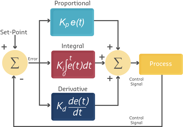
A PID controller uses three different control strategies simultaneously, each addressing different aspects of error correction:
- P (Proportional): Reacts to current error magnitude
- I (Integral): Reacts to accumulated error over time
- D (Derivative): Reacts to rate of error change
PID Controller Block Diagram: Error signal splits into three parallel paths. P term responds to current error, I term accumulates past errors, D term predicts future based on rate of change. All three combine to produce optimal control signal.
223.4 The PID Equation
\[ u(t) = K_p \cdot e(t) + K_i \cdot \int_{0}^{t} e(\tau) \, d\tau + K_d \cdot \frac{de(t)}{dt} \]
Where:
- \(u(t)\) = Controller output at time \(t\)
- \(e(t)\) = Error (Set Point - Process Variable)
- \(K_p\) = Proportional gain
- \(K_i\) = Integral gain
- \(K_d\) = Derivative gain
223.5 Understanding Error in PID Control
The foundation of PID control is the error signal:
- Process Variable (PV)
- The actual measured value of what we’re controlling (e.g., current temperature)
- Set Point (SP)
- The desired target value (e.g., target temperature)
- Error (e)
- The difference between desired and actual values
\[ e(t) = SP - PV(t) \]
NoteExample: Home Temperature Control
%%{init: {'theme': 'base', 'themeVariables': { 'primaryColor': '#2C3E50', 'primaryTextColor': '#fff', 'primaryBorderColor': '#16A085', 'lineColor': '#16A085', 'secondaryColor': '#E67E22', 'tertiaryColor': '#ecf0f1', 'fontSize': '14px'}}}%%
flowchart TB
    Start["Initial State:<br/>Room 18C<br/>Target 22C<br/>Error +4C"] --> P1["P: Strong Heat<br/>(Kp x 4)"]
    Start --> I1["I: Accumulating<br/>(Ki x integral)"]
    Start --> D1["D: Rate = 0<br/>(No change yet)"]

    P1 & I1 & D1 --> Heat1["Full Heating"]
    Heat1 --> Mid["After 5min:<br/>Room 20 deg C<br/>Error +2 deg C"]

    Mid --> P2["P: Medium Heat<br/>(Kp x 2)"]
    Mid --> I2["I: Growing<br/>(Ki x errors)"]
    Mid --> D2["D: Negative<br/>(Temp Rising)"]

    P2 & I2 & D2 --> Heat2["Reduced Heating"]
    Heat2 --> Final["After 15min:<br/>Room 22 deg C<br/>Error 0 deg C<br/>Stable"]

    style Start fill:#E67E22,stroke:#16A085,stroke-width:2px,color:#fff
    style Heat1 fill:#E74C3C,stroke:#2C3E50,stroke-width:2px,color:#fff
    style Heat2 fill:#16A085,stroke:#2C3E50,stroke-width:2px,color:#fff
    style Final fill:#2C3E50,stroke:#16A085,stroke-width:3px,color:#fff
PID Temperature Control Sequence: Initially large error (18 to 22C) produces full heating. As temperature rises, P term decreases (smaller error), D term provides braking (rapid approach), and system smoothly reaches setpoint without overshoot.
Scenario Analysis:
| Time | SP | PV | Error | Action |
|---|---|---|---|---|
| 0 min | 22C | 18C | +4C | Full heating |
| 5 min | 22C | 20C | +2C | Reduce heating |
| 10 min | 22C | 21.5C | +0.5C | Minimal heating |
| 15 min | 22C | 22C | 0C | Heating OFF |
| 20 min | 22C | 21.8C | +0.2C | Small heating pulse |
Key Observations:
- As error decreases, control action decreases
- Zero error means no action needed (maintain state)
- Small variations around set point are normal
223.6 Proportional Control (P)
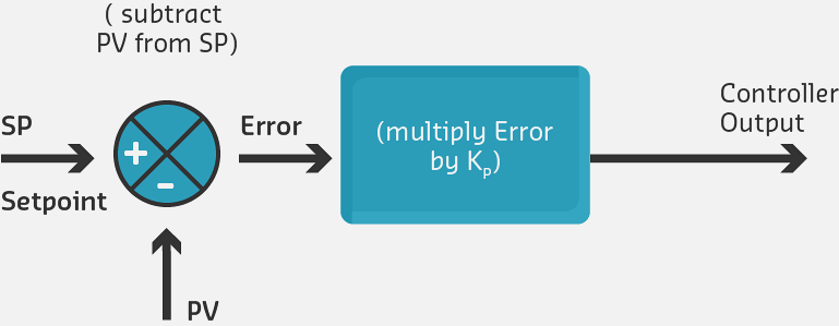
The Proportional term provides control action directly proportional to the current error. Larger errors produce stronger corrections.
\[ u_p(t) = K_p \cdot e(t) \]
%%{init: {'theme': 'base', 'themeVariables': { 'primaryColor': '#2C3E50', 'primaryTextColor': '#fff', 'primaryBorderColor': '#16A085', 'lineColor': '#16A085', 'secondaryColor': '#E67E22', 'tertiaryColor': '#ecf0f1', 'fontSize': '16px'}}}%%
graph LR
    Error["Error<br/>e(t)"] -->|Multiply by Kp| Gain["Proportional<br/>Gain<br/>Kp"]
    Gain -->|Output = Kp x e(t)| Output["Control<br/>Output<br/>u_p(t)"]

    Large["Large Error<br/>e = 5 deg C"] -.->|"Kp=2<br/>Output=10"| Strong["Strong<br/>Correction"]
    Small["Small Error<br/>e = 0.5 deg C"] -.->|"Kp=2<br/>Output=1"| Weak["Weak<br/>Correction"]

    style Error fill:#E67E22,stroke:#16A085,stroke-width:2px,color:#fff
    style Gain fill:#2C3E50,stroke:#16A085,stroke-width:3px,color:#fff
    style Output fill:#16A085,stroke:#2C3E50,stroke-width:2px,color:#fff
Characteristics:
- Fast response: Immediate reaction to errors
- Simple implementation: Single multiplication
- Proportional output: Big errors produce big corrections; small errors produce small corrections
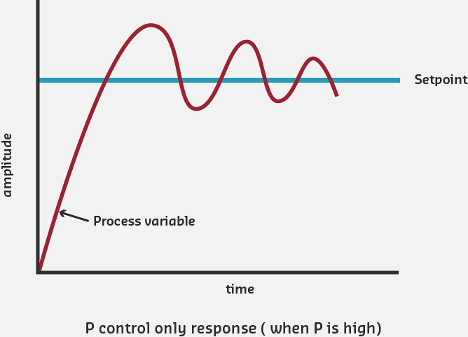
Problems with P-Only Control:
- Steady-State Error: System may never reach exact set point
- Overshoot: High Kp causes system to go past target
- Oscillation: High Kp can cause continuous cycling around set point
WarningP-Only Control Limitation: Steady-State Error
With proportional control alone, there’s often a permanent offset from the set point called steady-state error.
Why?
- As error decreases, control action decreases
- Eventually, control action becomes too weak to eliminate remaining error
- System settles with small persistent error
Example:
- Set point: 22C
- Steady state: 21.7C
- Error: 0.3C persists indefinitely
Solution: Add Integral control to eliminate steady-state error
223.7 Integral Control (I)
The Integral term accumulates error over time and provides control action based on the total accumulated error. This eliminates steady-state error that P-only control cannot handle.
\[ u_i(t) = K_i \cdot \int_{0}^{t} e(\tau) \, d\tau \]
%%{init: {'theme': 'base', 'themeVariables': { 'primaryColor': '#2C3E50', 'primaryTextColor': '#fff', 'primaryBorderColor': '#16A085', 'lineColor': '#16A085', 'secondaryColor': '#E67E22', 'tertiaryColor': '#ecf0f1', 'fontSize': '15px'}}}%%
graph TB
    Error["Error<br/>e(t)"] -->|Accumulate<br/>Over Time| Int["Integral<br/>sum of e(t)"]
    Int -->|Multiply by Ki| Gain["Integral<br/>Gain<br/>Ki"]
    Gain -->|Output = Ki x integral| Output["Control<br/>Output<br/>u_i(t)"]

    Persist["Persistent<br/>Small Error<br/>e = 0.5 deg C"] -.->|"Accumulates:<br/>0.5+0.5+0.5..."| Growing["Growing<br/>Integral<br/>Output"]
    Growing -.->|"Increases Until<br/>Error = 0"| Zero["Zero<br/>Steady-State<br/>Error"]

    style Error fill:#E67E22,stroke:#16A085,stroke-width:2px,color:#fff
    style Int fill:#2C3E50,stroke:#16A085,stroke-width:2px,color:#fff
    style Gain fill:#2C3E50,stroke:#16A085,stroke-width:2px,color:#fff
    style Output fill:#16A085,stroke:#2C3E50,stroke-width:2px,color:#fff
    style Zero fill:#16A085,stroke:#2C3E50,stroke-width:3px,color:#fff
How Integral Control Works:
- Accumulates error over time
- If error persists (even small error), integral grows
- Integral keeps increasing until error becomes zero
- Also called “automatic reset” - resets bias until error eliminated
Mathematical Intuition:
The integral accumulates (sums) all past errors:
Time | Error | Proportional | Integral Accumulated | Total Output
-----|-------|-------------|---------------------|-------------
0s   | +3C   | Kp×3 = 1.5  | 0                  | 1.5
1s   | +2C   | Kp×2 = 1.0  | Ki×(3+2) = 0.5     | 1.5
2s   | +1C   | Kp×1 = 0.5  | Ki×(3+2+1) = 0.6   | 1.1
3s   | +1C   | Kp×1 = 0.5  | Ki×(3+2+1+1) = 0.7 | 1.2
4s   | 0C    | Kp×0 = 0    | Ki×(...) = 0.7     | 0.7
5s   | 0C    | Kp×0 = 0    | Ki×(...) = 0.7     | 0.7

Kp = 0.5, Ki = 0.1
Key Observation: Even when P term drops to zero (error = 0), I term maintains output, compensating for disturbances.
Benefits of Adding Integral:
- Eliminates steady-state error: System reaches exact set point
- Compensates for disturbances: Overcomes constant external forces
- Automatic adjustment: No manual reset needed
223.8 Derivative Control (D)
The Derivative term provides control action based on the rate of change of error. It anticipates future error trends and provides damping to prevent overshoot.
\[ u_d(t) = K_d \cdot \frac{de(t)}{dt} \]
%%{init: {'theme': 'base', 'themeVariables': { 'primaryColor': '#2C3E50', 'primaryTextColor': '#fff', 'primaryBorderColor': '#16A085', 'lineColor': '#16A085', 'secondaryColor': '#E67E22', 'tertiaryColor': '#ecf0f1', 'fontSize': '15px'}}}%%
graph TB
    Error["Error<br/>e(t)"] -->|Calculate Rate<br/>of Change| Deriv["Derivative<br/>de(t)/dt"]
    Deriv -->|Multiply by Kd| Gain["Derivative<br/>Gain<br/>Kd"]
    Gain -->|Output = Kd x de/dt| Output["Control<br/>Output<br/>u_d(t)"]

    Fast["Error Decreasing<br/>Rapidly<br/>de/dt = -2 deg C/s"] -.->|Negative<br/>Derivative| Brake["Negative Output<br/>(Reduce Control)<br/>Prevents Overshoot"]
    Slow["Error Stable<br/>de/dt = 0"] -.->|Zero<br/>Derivative| None["No D<br/>Contribution"]

    style Error fill:#E67E22,stroke:#16A085,stroke-width:2px,color:#fff
    style Deriv fill:#2C3E50,stroke:#16A085,stroke-width:2px,color:#fff
    style Gain fill:#2C3E50,stroke:#16A085,stroke-width:2px,color:#fff
    style Output fill:#16A085,stroke:#2C3E50,stroke-width:2px,color:#fff
    style Brake fill:#16A085,stroke:#2C3E50,stroke-width:3px,color:#fff
How Derivative Control Works:
- Measures how fast error is changing: de/dt
- If error decreasing rapidly, derivative is negative
- Negative derivative reduces control action (anticipates reaching target)
- Provides damping effect to prevent overshoot
- Acts as predictive brake
Benefits of Adding Derivative:
- Reduces overshoot: Dampens aggressive P and I responses
- Improves stability: Prevents oscillations
- Faster settling: Reaches steady state more quickly
- Better response to changing conditions: Anticipates trends
Cautions with Derivative:
- Noise sensitivity: Amplifies high-frequency noise in sensor readings
- Difficult to tune: Kd selection is challenging
- Rarely used alone: Almost always combined with P and/or I
223.9 PID Configurations Comparison
%%{init: {'theme': 'base', 'themeVariables': { 'primaryColor': '#2C3E50', 'primaryTextColor': '#fff', 'primaryBorderColor': '#16A085', 'lineColor': '#16A085', 'secondaryColor': '#E67E22', 'tertiaryColor': '#ecf0f1', 'fontSize': '14px'}}}%%
graph LR
    subgraph POnly ["P-Only"]
        P1["Fast<br/>Response"] --> P2["Steady-State<br/>Error<br/>Remains"]
    end

    subgraph PI ["PI Control"]
        I1["Good<br/>Response"] --> I2["Zero<br/>Steady-State<br/>Error"]
        I2 --> I3["Possible<br/>Overshoot"]
    end

    subgraph PID ["PID Control"]
        D1["Fast<br/>Response"] --> D2["Zero<br/>Steady-State<br/>Error"]
        D2 --> D3["Minimal<br/>Overshoot<br/>Best Performance"]
    end

    style P2 fill:#E74C3C,stroke:#2C3E50,stroke-width:2px,color:#fff
    style I3 fill:#E67E22,stroke:#16A085,stroke-width:2px,color:#fff
    style D3 fill:#16A085,stroke:#2C3E50,stroke-width:3px,color:#fff
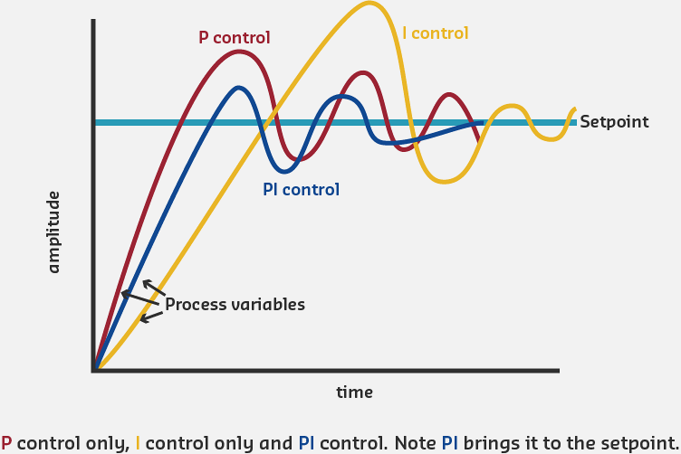
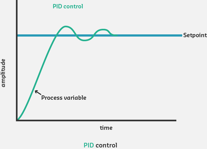
PID Configuration Performance Comparison: P-only provides fast response but leaves steady-state error. PI eliminates error but may overshoot. Full PID combines fast response, zero error, and minimal overshoot.
| Mode | Usage | Application Examples |
|---|---|---|
| P | Sometimes | Simple temperature control, LED brightness |
| PI | Most common | HVAC systems, level control, pressure regulation |
| PID | Sometimes | Motor speed control, precision positioning |
| PD | Rare | Servo motors, fast response systems |
NoteAlternative View: PID Terms as Time Perspectives
%%{init: {'theme': 'base', 'themeVariables': { 'primaryColor': '#2C3E50', 'primaryTextColor': '#fff', 'primaryBorderColor': '#16A085', 'lineColor': '#16A085', 'secondaryColor': '#E67E22', 'tertiaryColor': '#7F8C8D', 'fontSize': '12px'}}}%%
graph LR
    subgraph Past["PAST (Integral Term)"]
        direction TB
        I_Desc["Remembers all<br/>previous errors"]
        I_Calc["∫ e(τ) dτ"]
        I_Benefit["Eliminates<br/>steady-state error"]
        I_Risk["⚠️ Can cause<br/>overshoot if too high"]
    end

    subgraph Present["PRESENT (Proportional Term)"]
        direction TB
        P_Desc["Responds to<br/>current error"]
        P_Calc["Kp × e(t)"]
        P_Benefit["Immediate<br/>correction"]
        P_Risk["⚠️ Cannot eliminate<br/>persistent error alone"]
    end

    subgraph Future["FUTURE (Derivative Term)"]
        direction TB
        D_Desc["Predicts based on<br/>rate of change"]
        D_Calc["de/dt"]
        D_Benefit["Prevents<br/>overshoot"]
        D_Risk["⚠️ Sensitive to<br/>sensor noise"]
    end

    Past -->|"Ki ×"| Sum["Σ<br/>Combined<br/>Output"]
    Present -->|"Kp ×"| Sum
    Future -->|"Kd ×"| Sum

    Sum --> Plant["System<br/>Response"]

    style Past fill:#7F8C8D,stroke:#2C3E50,color:#fff
    style Present fill:#E67E22,stroke:#2C3E50,color:#fff
    style Future fill:#16A085,stroke:#2C3E50,color:#fff
    style Sum fill:#2C3E50,stroke:#16A085,color:#fff
223.10 Knowledge Check
223.11 Summary
This chapter covered the theory of PID control:
- PID Equation: Combined P, I, and D terms with their respective gains
- Proportional (P): Responds to current error magnitude - fast but leaves steady-state error
- Integral (I): Accumulates past errors - eliminates steady-state error but can cause windup
- Derivative (D): Predicts future from rate of change - reduces overshoot but sensitive to noise
- Configuration Selection: P for simple systems, PI for most applications, full PID for precision control
223.12 What’s Next
The next chapter covers PID Tuning and Applications, including systematic tuning methods, real-world examples, and practical implementation considerations for IoT systems.
NoteRelated Chapters
- Feedback Fundamentals - Foundation concepts
- Open-Loop and Closed-Loop Systems - Control architectures
- PID Tuning and Applications - Practical implementation
- Sensor Fundamentals - Feedback sensors
- Actuators - Control outputs