371  Sensor Node Characteristics

371.1 Learning Objectives

By the end of this chapter, you will be able to:

• Describe hardware components: Explain the four subsystems of sensor nodes (sensing, processing, communication, power)
• Analyze resource constraints: Quantify energy, memory, and computational limitations in WSN design
• Explain multi-hop communication: Calculate energy savings from the radio power law
• Compare WSN vs traditional networks: Identify fundamental differences in scale, economics, and constraints
• Classify node types: Distinguish between regular, cluster head, gateway, actuator, and mobile nodes
• Apply worked examples: Analyze energy hotspot problems and recommend mitigation strategies

---

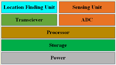
371.2 Characteristics of Sensor Nodes

⏱️ ~12 min | ⭐⭐ Intermediate | 📋 P05.C31.U02

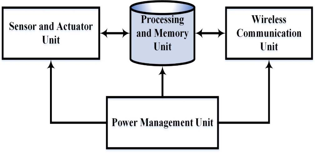
Sensor nodes are the fundamental building blocks of WSNs, each comprising several key components that enable autonomous sensing, processing, and communication.

371.2.1 Hardware Components

371.2.1.1 Sensor Node Architecture

A sensor node consists of four key subsystems working together to enable autonomous sensing and communication:

Subsystem	Components	Power Draw	Function
Sensing	ADC, sensors	1-10 mW	Data acquisition from environment
Processing	MCU, memory	10-100 mW	Local computation, protocol execution
Communication	Radio, antenna	50-300 mW	Data transmission/reception
Power	Battery, harvester	N/A	Energy supply and management

NotePower Distribution Reality

The communication subsystem typically consumes 3-30× more power than sensing and processing combined. This fundamental asymmetry drives WSN protocol design toward minimizing radio usage through duty cycling, data aggregation, and local processing.

%% fig-alt: "Sensor node architecture block diagram showing four subsystems: Sensing Unit (sensors and ADC), Processing Unit (microcontroller and memory), Communication Unit (radio transceiver and antenna), and Power Unit (battery and voltage regulator) - all interconnected with communication subsystem consuming most power"
%%{init: {'theme': 'base', 'themeVariables': { 'primaryColor': '#2C3E50', 'primaryTextColor': '#fff', 'primaryBorderColor': '#16A085', 'lineColor': '#16A085', 'secondaryColor': '#E67E22', 'tertiaryColor': '#7F8C8D', 'fontSize': '14px'}}}%%
flowchart TB
    subgraph NODE["Sensor Node Architecture"]
        subgraph SENSE["Sensing Unit<br/>(1-10 mW)"]
            S1[Temperature<br/>Sensor] --> ADC[ADC]
            S2[Humidity<br/>Sensor] --> ADC
            S3[Light<br/>Sensor] --> ADC
        end
        subgraph PROC["Processing Unit<br/>(10-100 mW)"]
            ADC --> MCU[Microcontroller<br/>8-32 bit]
            MCU <--> MEM[Memory<br/>KB-MB]
        end
        subgraph COMM["Communication Unit<br/>(50-300 mW)"]
            MCU <--> RADIO[Radio<br/>Transceiver<br/>802.15.4/BLE]
            RADIO <--> ANT[Antenna]
        end
        subgraph PWR["Power Unit"]
            BAT[Battery<br/>mAh-Ah] --> REG[Voltage<br/>Regulator]
            HARVEST[Energy<br/>Harvester<br/>Optional] -.-> BAT
            REG --> |Powers all units| MCU
            REG --> |Powers all units| ADC
            REG --> |Powers all units| RADIO
        end
    end

    style SENSE fill:#2C3E50,stroke:#16A085,color:#fff
    style PROC fill:#2C3E50,stroke:#16A085,color:#fff
    style COMM fill:#E67E22,stroke:#16A085,color:#fff
    style PWR fill:#16A085,stroke:#2C3E50,color:#fff
    style NODE fill:#7F8C8D,stroke:#2C3E50,color:#fff

Figure 371.1: Sensor node architecture block diagram showing four subsystems: Sensing Unit (sensors and ADC), Processing Unit (microcontroller and memory), Communication Unit (radio transceiver), and Power Unit (battery). {fig-alt=“Block diagram of sensor node with four color-coded subsystems: Sensing Unit in navy showing temperature, humidity, and light sensors feeding into ADC; Processing Unit showing microcontroller connected to memory; Communication Unit highlighted in orange showing radio transceiver and antenna consuming 50-300mW; Power Unit in teal showing battery and optional energy harvester powering all components”}

%% fig-alt: "Energy consumption timeline showing sensor node duty cycle with sleep, sense, process, and transmit phases"
%%{init: {'theme': 'base', 'themeVariables': { 'primaryColor': '#2C3E50', 'primaryTextColor': '#fff', 'primaryBorderColor': '#16A085', 'lineColor': '#16A085', 'secondaryColor': '#E67E22', 'tertiaryColor': '#7F8C8D', 'fontSize': '13px'}}}%%
gantt
    title Sensor Node Duty Cycle - Energy Over Time
    dateFormat X
    axisFormat %s

    section Power State
    Sleep (0.01mW)           :done, sleep1, 0, 900
    Wake & Sense (5mW)       :active, sense, 900, 920
    Process Data (50mW)      :crit, proc, 920, 940
    Transmit (200mW)         :crit, tx, 940, 960
    Sleep (0.01mW)           :done, sleep2, 960, 1000

    section Energy Used
    Sleep: 0.009 mJ          :done, e1, 0, 900
    Sense: 0.1 mJ            :active, e2, 900, 920
    Process: 1.0 mJ          :crit, e3, 920, 940
    Transmit: 4.0 mJ         :crit, e4, 940, 960

Figure 371.2: Energy Timeline View: This Gantt chart shows a typical 1-second duty cycle where the node sleeps for 900ms (consuming only 0.009 mJ), wakes to sense for 20ms, processes locally for 20ms, and transmits for 20ms. Despite transmission being only 2% of the cycle time, it consumes 78% of the energy (4.0 mJ out of 5.1 mJ total). This visualization helps students understand why WSN protocols focus obsessively on minimizing radio transmissions. {fig-alt=“Gantt chart showing sensor node 1-second duty cycle with four phases: Sleep period of 900ms consuming 0.01mW (0.009 mJ energy), Wake and Sense period of 20ms at 5mW (0.1 mJ), Process Data period of 20ms at 50mW (1.0 mJ), and Transmit period of 20ms at 200mW (4.0 mJ) - demonstrating that transmission uses 78% of total energy despite being only 2% of cycle time”}

Figure 371.3: Basic components of a sensor node - microcontroller, radio transceiver, sensors, memory, and power supply

NoteAcademic Reference: WSN Node Architecture (IIT Kharagpur NPTEL)

Wireless sensor node architecture showing key components

Source: IIT Kharagpur - NPTEL Introduction to Internet of Things

Figure 371.4: Examples of sensor nodes showing various form factors and capabilities

Sensing Unit: - Sensors: Transduce physical phenomena into electrical signals (temperature, humidity, light, pressure, accelerometer, etc.) - Analog-to-Digital Converter (ADC): Converts analog sensor readings to digital values for processing - Multiple Sensor Integration: Modern nodes often integrate multiple sensor types (multi-modal sensing)

Processing Unit: - Microcontroller (MCU): Executes application logic, protocols, and data processing - Typical Specifications: 8-16 bit processors, MHz clock speeds, KB-MB RAM, KB-MB flash memory - Examples: ARM Cortex-M series, TI MSP430, Atmel AVR, Arduino platforms

Communication Unit: - Radio Transceiver: Enables wireless communication with other nodes - Common Standards: IEEE 802.15.4, Bluetooth Low Energy (BLE), LoRa, Sub-GHz radios - Antenna: Internal or external for signal transmission/reception - Typical Range: 10-100 meters (short-range), up to several kilometers (long-range LPWAN)

Power Supply: - Primary Batteries: Non-rechargeable (AA, coin cells), long lifetime but limited capacity - Rechargeable Batteries: Li-ion, Li-polymer, enabling solar or energy harvesting recharge - Energy Harvesting: Solar panels, vibration harvesters, thermal energy, RF energy harvesting - Typical Capacity: mAh to few Ah, determining operational lifetime

Optional Components: - Storage: SD cards or flash memory for local data logging - Positioning: GPS modules for location awareness (power-intensive) - Actuators: Enable control functions (valves, motors, switches) - Security: Cryptographic co-processors for secure communication

371.2.2 Node Capabilities

Sensing Capabilities: - Measurement accuracy and precision - Sampling frequency and resolution - Multi-modal sensing (combining multiple sensor types) - Calibration and drift management

Processing Capabilities: - Data preprocessing and filtering - Feature extraction and compression - Local decision making - In-network data aggregation

Communication Capabilities: - Data transmission rates (typically kbps to hundreds of kbps) - Communication range (meters to kilometers) - Multi-hop routing support - Protocol support (MAC, routing, transport layers)

Energy Capabilities: - Battery capacity and type - Power consumption profiles (active, sleep, deep sleep modes) - Energy harvesting potential - Expected operational lifetime

371.2.3 Multi-hop Communication

Multi-hop routing is a fundamental characteristic of WSNs, enabling nodes beyond direct radio range to communicate by relaying messages through intermediate nodes.

Figure 371.5: Multi-hop routing path in WSN showing data forwarding from source to sink through intermediate nodes

371.2.3.1 Why Multi-hop? The Radio Power Law

Radio transmission power follows the path loss model where required power scales with distance:

\[P_{tx} \propto d^n\]

where: - \(P_{tx}\) = transmission power - \(d\) = distance to receiver - \(n\) = path loss exponent (typically 2-4 for wireless propagation)

Energy Benefit Example:

Consider transmitting data 100 meters to a sink:

Approach	Path Loss (n=2)	Path Loss (n=4)	Relative Energy
Direct: 1 hop × 100m	\(100^2 = 10,000\)	\(100^4 = 100,000,000\)	1× (baseline)
Multi-hop: 10 hops × 10m	\(10 \times 10^2 = 1,000\)	\(10 \times 10^4 = 100,000\)	10× savings (n=2) 1000× savings (n=4)

ImportantThe Multi-hop Energy Paradox

While multi-hop routing dramatically reduces per-hop transmission power, it introduces three critical trade-offs:

1. Latency Increase: Each hop adds processing and queuing delay. A 10-hop path with 10ms per-hop delay = 100ms total vs. 10ms for direct transmission.

2. Intermediate Node Burden: Nodes near the sink relay massive traffic from all downstream nodes, depleting batteries 10-100× faster (the “hotspot problem”).

3. Routing Overhead: Maintaining multi-hop routes requires periodic control messages, topology discovery, and route repair mechanisms that consume energy and bandwidth.

Solution: Use multi-hop routing strategically—essential for long-range communication beyond single-hop radio range, but avoid unnecessary hops. Deploy multiple sinks to reduce average hop count, implement energy-aware routing to balance load, and use adaptive transmission power control to optimize per-hop distances.

371.2.3.2 Multi-hop Trade-offs

Advantages: - Extended Range: Coverage beyond single-hop radio limits - Lower Transmission Power: Reduced per-hop energy consumption - Redundancy: Multiple paths increase reliability - Scalability: Supports large deployments

Challenges: - Higher Latency: Each hop adds delay (10-50 ms typical per hop) - Increased Complexity: Routing protocols, topology maintenance - Hotspot Problem: Nodes near sink relay all traffic - Overhead: Routing messages consume energy and bandwidth

Practical Design Guidelines:

1. Minimize Hop Count: Deploy sufficient gateways to keep average path length < 5 hops
2. Balance Energy: Use energy-aware routing to avoid overloading specific nodes
3. Adaptive Transmission Power: Adjust radio power based on required hop distance
4. Hierarchical Topologies: Cluster-based architectures reduce long multi-hop chains

371.2.4 WSN vs. Traditional Networks

Wireless Sensor Networks differ fundamentally from conventional computer networks in scale, economics, and operational constraints:

Aspect	Traditional Network	WSN
Node Cost	$100-1000+ per device	$1-10 per node
Node Count	10s-100s devices	100s-10,000s nodes
Deployment	Planned, structured	Ad-hoc, dense, unplanned
Power Source	Wired AC or rechargeable	Battery (months-years), harvesting
Data Flow	Any-to-any, peer-to-peer	Many-to-one (convergecast to sink)
Lifetime	Years with maintenance	Months-years, unattended
Bandwidth	Mbps-Gbps	kbps-100s kbps
Processing	GHz multi-core CPUs	MHz 8-32 bit MCUs
Memory	GB RAM, TB storage	KB RAM, MB flash
QoS	Guaranteed latency/bandwidth	Best-effort, graceful degradation
Security	Centralized PKI, strong crypto	Lightweight crypto, resource-constrained
Mobility	Limited (laptops, phones)	Mostly static, some mobile sinks/nodes
Address Assignment	DHCP, static IP	Auto-configuration, hierarchical IDs
Network Discovery	Manual configuration	Self-organizing, distributed

TipWhy These Differences Matter for Design

Traditional network assumptions break in WSNs:

1. IP-Based Protocols Too Heavy: Full TCP/IP stack requires 50-100 KB flash + KB RAM—exceeding many sensor node capabilities. Solutions: 6LoWPAN (compressed IPv6), CoAP (lightweight HTTP alternative).

2. Always-On Radio Assumption: Traditional protocols assume devices listen continuously. WSNs use duty cycling (1-10% radio active) to extend battery life 10-100×, requiring asynchronous MAC protocols.

3. Reliability Through Retransmission: TCP’s reliable delivery via ACKs and retransmissions is energy-prohibitive in WSNs where radio dominates power. WSNs use redundancy (multiple sensors measure same phenomenon) and in-network aggregation instead.

4. End-to-End Addressing: Traditional networks address individual devices. WSNs often use data-centric routing (query “get temperature > 30°C from Region A”) where specific node identity is irrelevant—only data matters.

5. Centralized Management: Traditional networks rely on SNMP, centralized controllers. WSNs require distributed, autonomous operation due to limited connectivity to management infrastructure.

Design for WSN constraints: minimize radio transmissions, use application-specific protocols, embrace statistical aggregation over perfect reliability, deploy redundancy at the sensing layer (cheap nodes) rather than network layer (expensive protocols).

371.2.5 Resource Constraints

Energy Constraints: The most critical limitation in WSNs. Radio communication typically consumes the most energy, followed by sensing and processing.

Typical Power Consumption: - Active mode (sensing + transmitting): 10-50 mW - Idle listening: 1-20 mW - Sleep mode: 1-100 μW - Deep sleep: < 1 μW

Memory Constraints: - RAM: 2 KB - 64 KB (working memory) - Flash/ROM: 32 KB - 512 KB (program and data storage) - Impact: Limits code complexity, buffering, and local storage

Computational Constraints: - Processor Speed: 1-48 MHz typical - Computation: Simple arithmetic, limited cryptography, basic signal processing - Impact: Complex algorithms must be simplified or offloaded

Communication Constraints: - Bandwidth: Typically 20-250 kbps (802.15.4), up to 1 Mbps (BLE) - Range: Limited by power and frequency - Reliability: Subject to interference, obstacles, and environmental factors

WarningIdle Listening Drains Batteries Faster Than You Think

Many WSN deployments fail because developers underestimate idle listening power consumption. A sensor node with its radio in idle listening mode (waiting to receive) consumes 10-20 mW continuously - nearly as much as actively transmitting! In a network with 1% duty cycle, idle listening can waste 90% of total energy. For example, a 2000 mAh battery at 15 mA idle current lasts only 5.5 days, but with proper duty cycling (1% active) extends to 18 months. Solution: Implement aggressive duty cycling with synchronized sleep schedules (S-MAC), use low-power listening with preamble sampling (B-MAC), or deploy wake-up radio receivers that consume only microamps while monitoring for incoming messages.

NoteWorked Example: Multi-Hop Energy Hotspot Analysis

Scenario: A forest monitoring WSN has 100 temperature sensors arranged in a 10x10 grid, each 50 meters apart. The gateway is at one corner. After 6 months, nodes near the gateway fail while edge nodes still have 70% battery. Analyze the energy hotspot problem and design a mitigation strategy.

Given:

• Grid size: 10×10 nodes, 50m spacing (500m × 500m field)
• Gateway at position (0,0)
• Radio range: 75m (allows diagonal hops)
• Data rate: Each node transmits 1 packet/hour (own data)
• Packet size: 50 bytes
• TX energy: 50 µJ/byte, RX energy: 30 µJ/byte
• Battery: 2000 mAh at 3.3V = 23.76 kJ

Steps:

1. Calculate hop count for each node position:
   • Node at (9,9): 6 hops to gateway (diagonal path)
   • Node at (0,9): 9 hops (vertical path)
   • Average hop count: ~5 hops across network
2. Calculate traffic load at gateway-adjacent nodes:
   • Nodes at (0,1), (1,0), (1,1) relay traffic from entire network
   • Total network packets: 100 nodes × 1 packet/hour = 100 packets/hour
   • Node (1,1) relays approximately 60% of traffic = 60 packets/hour
   • Node’s own packet: 1 packet/hour
   • Total: 61 packets/hour for hotspot node vs. 1 packet/hour for edge node
3. Calculate energy consumption difference:
   • Edge node energy/hour: 1 packet × 50 bytes × 50 µJ = 2.5 mJ
   • Hotspot node energy/hour:
     • TX own data: 50 bytes × 50 µJ = 2.5 mJ
     • TX relayed: 60 × 50 × 50 µJ = 150 mJ
     • RX relayed: 60 × 50 × 30 µJ = 90 mJ
     • Total: 242.5 mJ/hour (97× more than edge node)
4. Calculate battery lifetime disparity:
   • Edge node lifetime: 23,760,000 mJ / 2.5 mJ/hour = 9,504,000 hours = 1,085 years (theoretical)
   • Hotspot node lifetime: 23,760,000 mJ / 242.5 mJ/hour = 97,979 hours = 11.2 years
   • With realistic 10% duty cycle overhead: Edge = 10+ years, Hotspot = 1.1 years
5. Design mitigation: Deploy 4 gateways:
   • Place gateways at (0,0), (0,9), (9,0), (9,9)
   • Maximum hop count reduced from 6 to 3
   • Maximum relay load per node: 25% of network = 25 packets/hour
   • New hotspot energy: ~65 mJ/hour (74% reduction)

Result: Adding 3 additional gateways reduces worst-case relay burden by 74%, extending hotspot node lifetime from 1.1 years to 4+ years while edge nodes remain unaffected.

Key Insight: In convergecast WSNs, nodes near the sink experience traffic proportional to the entire network size. Gateway placement and quantity are critical design decisions - the cost of additional gateways is often far less than the cost of replacing depleted batteries in hard-to-access hotspot locations.

NoteWorked Example: Choosing Between Battery and Energy Harvesting

Scenario: An environmental agency needs to deploy 50 air quality sensors on streetlights in a city center for 5-year continuous monitoring. Compare battery-only versus solar harvesting approaches and recommend the most cost-effective solution.

Given:

• Deployment: 50 sensors on streetlight poles (partial shading)
• Required lifetime: 5 years (43,800 hours)
• Average power consumption: 250 µW (after optimization with 0.5% duty cycle)
• Location: Northern European city (limited winter sunlight: 2 hours/day December)
• Solar panel efficiency in urban canyon: 40% of rated due to shading
• Maintenance cost: $150/visit (cherry picker + technician)

Steps:

1. Calculate battery-only requirements: \[\text{Energy needed} = 250 \mu W \times 43800 \text{ hours} = 10.95 \text{ Wh}\]

   • Primary lithium battery: 3.6V × 19Ah = 68.4 Wh (Tadiran TL-5930)
   • Cost per battery: $45
   • Available energy margin: 6.2× safety factor (accounts for self-discharge, temperature)

2. Calculate solar harvesting system:

   • Winter minimum: 2 hours × 40% efficiency = 0.8 effective sun-hours/day
   • Required harvest rate: 250 µW × 24h / 0.8h = 7.5 mW panel output
   • With 50% harvesting efficiency: 15 mW panel needed
   • Small solar panel (50×50mm): $8, provides 100 mW peak = 10 mW urban effective
   • Need 2× panels: $16
   • Battery for 3 days backup: 250 µW × 72h = 18 mWh → 50 mAh LiPo: $5
   • Charge controller: $12
   • Total harvesting BOM: $33

3. Calculate 5-year total cost comparison:

   Approach	Initial Cost	5-Year Maintenance	Total per Node
   Battery-only	$45	$0 (no visits)	$45
   Solar harvest	$33	$150 × 0.5 visits (panel cleaning)	$108

4. Factor in failure modes:

   • Battery failure rate: 1% over 5 years (lithium primary very reliable)
   • Solar system failure rate: 15% (panel damage, connector corrosion, controller failure)
   • Battery-only: 50 × $45 + 0.5 replacement visits × $150 = $2,325
   • Solar: 50 × $33 + 7.5 failures × $150 repair + 25 cleanings × $150 = $5,655

Result: For this 5-year deployment with low power consumption (250 µW), battery-only is 2.4× more cost-effective than solar harvesting. The high-quality primary lithium battery provides reliable, maintenance-free operation.

Key Insight: Energy harvesting is not always the best choice. For deployments under 10 years with very low power budgets (<1 mW average), high-capacity primary batteries often provide better reliability and lower total cost of ownership than harvesting systems. Reserve harvesting for: (1) >10 year deployments, (2) >1 mW average power, or (3) locations where battery replacement is physically impossible.

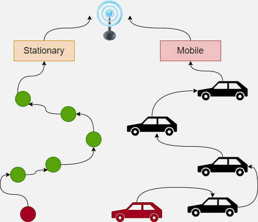
371.2.6 Node Types and Roles

Regular Sensor Nodes: - Most common and numerous - Perform sensing and basic routing - Minimal configuration and capabilities

Cluster Head Nodes: - Coordinate groups of sensor nodes - Aggregate and forward data - More capable hardware and energy resources - May be rotated among nodes to balance energy consumption

Gateway/Sink Nodes: - Interface between WSN and external networks - More powerful processing and communication - Often mains-powered - Bridge different protocols and networks

Sink Node Architecture

Figure 371.6: Sink node architecture illustrating the gateway’s role in bridging sensor networks to external infrastructure.

Actuator Nodes: - Include actuation capabilities - Respond to sensed conditions or commands - Examples: irrigation valves, motors, heaters

Mobile Nodes: - Mounted on vehicles, robots, or carried by people - Dynamic topology challenges - Data collection through mobility (data mules)

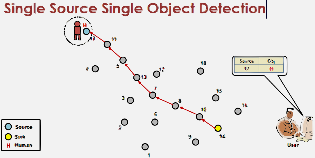
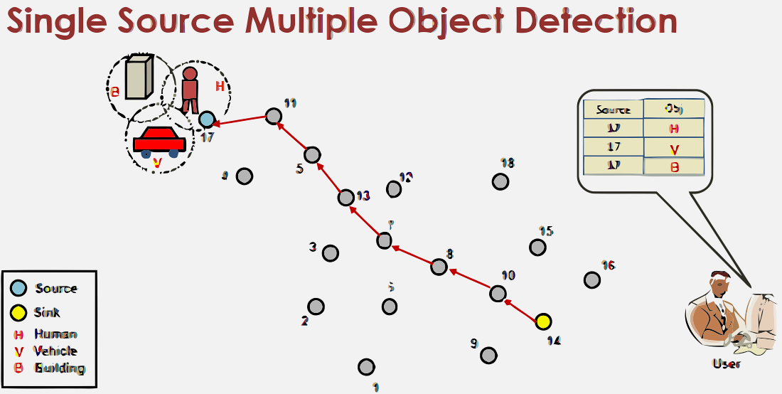
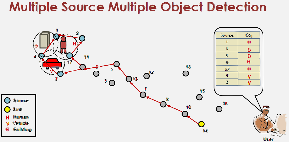
371.2.7 Detection Scenarios

Understanding how sensor nodes detect targets is fundamental to WSN design:

Figure 371.7: Single source single object detection in WSN - one sensor detecting one target

Figure 371.8: Single source multiple object detection - one sensor tracking multiple targets simultaneously

Figure 371.9: Multiple source single object detection - collaborative sensing of one target by multiple sensors

Figure 371.10: Multiple source multiple object detection - distributed sensing network tracking multiple targets

371.3 Summary

This chapter covered sensor node characteristics essential for WSN design:

• Hardware Architecture: Four subsystems (sensing, processing, communication, power) with radio communication consuming 3-30× more power than other components
• Multi-hop Communication: The radio power law (\(P \propto d^n\)) makes multi-hop routing dramatically more energy-efficient, but introduces latency and hotspot challenges
• WSN vs Traditional Networks: Fundamental differences in cost ($1-10 vs $100+), scale (100s-10,000s nodes), power (battery vs mains), and data flow (many-to-one vs any-to-any)
• Resource Constraints: Severe limitations in energy (mAh batteries), memory (KB RAM), computation (MHz processors), and bandwidth (kbps)
• Node Types: Regular sensors, cluster heads, gateways, actuators, and mobile nodes each serve different roles in network operation
• Energy Hotspots: Nodes near the sink relay all traffic, requiring strategic gateway placement and energy-aware routing

371.4 What’s Next

Continue to Emergent Swarm Behavior to explore how simple local rules create intelligent network-wide behaviors through Reynolds’ Boids model and its applications to coverage optimization, self-healing, and distributed coordination.