%%{init: {'theme': 'base', 'themeVariables': { 'primaryColor': '#2C3E50', 'primaryTextColor': '#fff', 'primaryBorderColor': '#16A085', 'lineColor': '#16A085', 'secondaryColor': '#E67E22', 'tertiaryColor': '#ecf0f1', 'fontSize': '15px'}}}%%
flowchart LR
    SP["Target:<br/>22 deg C"] --> Comp["Compare"]
    Sensor["Temperature<br/>Sensor:<br/>21 deg C"] --> Comp
    Comp -->|Error: +1 deg C<br/>Need Heat| MCU["Smart<br/>Thermostat<br/>Controller"]
    MCU -->|Activate| Heater["Heating<br/>System"]
    Heater -->|Warm Air| Room["Room<br/>Environment"]
    Room -.->|Measure<br/>Temperature| Sensor

    style SP fill:#16A085,stroke:#2C3E50,stroke-width:2px,color:#fff
    style Comp fill:#E67E22,stroke:#16A085,stroke-width:2px,color:#fff
    style MCU fill:#2C3E50,stroke:#16A085,stroke-width:2px,color:#fff
    style Heater fill:#E67E22,stroke:#16A085,stroke-width:2px,color:#fff
    style Sensor fill:#2C3E50,stroke:#16A085,stroke-width:2px,color:#fff
    style Room fill:#7F8C8D,stroke:#16A085,stroke-width:2px,color:#fff
222 PID: Open-Loop and Closed-Loop Systems
222.1 Learning Objectives
By the end of this chapter, you will be able to:
- Distinguish Control Types: Compare open-loop and closed-loop control strategies and their applications
- Identify System Characteristics: Recognize advantages and disadvantages of each control approach
- Apply Decision Frameworks: Use systematic criteria to select appropriate control architecture
- Design IoT Control Systems: Choose between local edge control and cloud-based control loops
TipMVU: Minimum Viable Understanding
Core concept: Open-loop systems execute predetermined actions blindly (like a timer), while closed-loop systems continuously monitor output and adjust (like a thermostat). Why it matters: Closed-loop systems can self-correct errors and adapt to disturbances, but require sensors and more complexity. Key takeaway: Most IoT control applications benefit from closed-loop feedback, but simple monitoring-only devices may operate open-loop at the device level while the overall system implements feedback through cloud coordination.
222.2 Prerequisites
Before diving into this chapter, you should be familiar with:
- Feedback Fundamentals: Understanding feedback concepts, negative vs positive feedback, and IoT applications
- Sensor Fundamentals: Sensor characteristics for feedback measurement
- Actuators: Control outputs for implementing corrections
222.3 Closed-Loop Feedback Systems
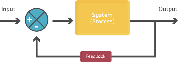
In a closed-loop system, a portion of the output is fed back to the input and either added to (positive feedback) or subtracted from (negative feedback) the input signal. This creates a self-regulating system that continuously updates based on current output conditions.

Closed-Loop Feedback System Block Diagram: Set point is compared with measured output, generating error signal. Controller processes error and adjusts system input. Feedback sensor creates continuous regulation loop.
Key Components:
- Set Point (SP): The desired target value
- Error Signal: Difference between set point and measured output
- Controller: Processes error and determines corrective action
- Process/Plant: The system being controlled
- Feedback Sensor: Measures actual output
- Comparator: Computes error = SP - measured value
NoteExample: Smart Home Heating System
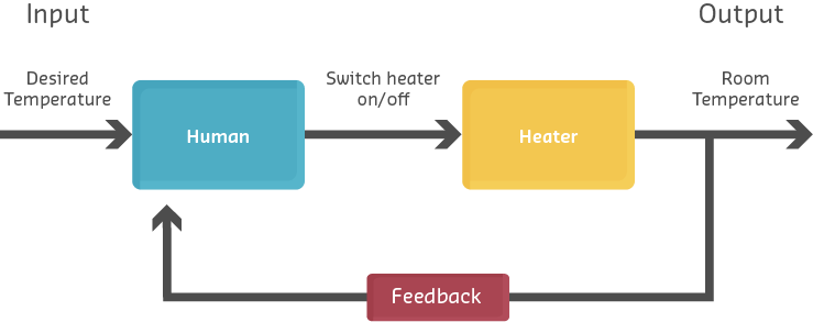
Smart Home Heating Control Loop: Thermostat compares target (22C) with measured temperature (21C), calculates error (+1C), activates heater, and continuously monitors room temperature to maintain setpoint.
Operation:
- User sets desired temperature: 22C
- Temperature sensor measures actual temperature: 21C
- Error = 22C - 21C = +1C
- Controller activates heating system
- Room temperature rises toward 22C
- As error decreases, heating output adjusts
- System maintains temperature within tolerance
222.4 Open-Loop Control Systems
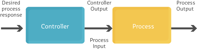
An open-loop system does not monitor or measure its output. It executes a predetermined action based solely on the input, without feedback. This is also called a non-feedback system.
%%{init: {'theme': 'base', 'themeVariables': { 'primaryColor': '#2C3E50', 'primaryTextColor': '#fff', 'primaryBorderColor': '#16A085', 'lineColor': '#16A085', 'secondaryColor': '#E67E22', 'tertiaryColor': '#ecf0f1', 'fontSize': '16px'}}}%%
graph LR
    Input["Input<br/>(Set Timer<br/>60 min)"] --> Controller["Controller<br/>(Timer)"]
    Controller -->|Run for<br/>60 minutes| Process["Process<br/>(Dryer)"]
    Process -->|Unknown State| Output["Output<br/>(Clothes)"]

    style Input fill:#16A085,stroke:#2C3E50,stroke-width:2px,color:#fff
    style Controller fill:#2C3E50,stroke:#16A085,stroke-width:2px,color:#fff
    style Process fill:#E67E22,stroke:#16A085,stroke-width:2px,color:#fff
    style Output fill:#7F8C8D,stroke:#16A085,stroke-width:2px,color:#fff
Open-Loop System Block Diagram: Input (timer setting) determines controller action without measuring output state. System executes predetermined sequence with no knowledge of actual results.
Characteristics:
- No feedback path from output to input
- Cannot self-correct for disturbances or errors
- Simpler and less expensive to implement
- Suitable when output is predictable and disturbances are minimal
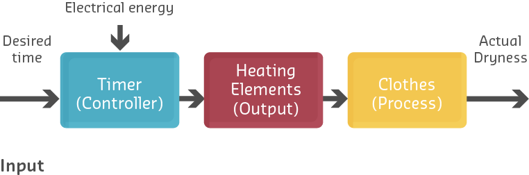
NoteExample: Automatic Clothes Dryer
%%{init: {'theme': 'base', 'themeVariables': { 'primaryColor': '#2C3E50', 'primaryTextColor': '#fff', 'primaryBorderColor': '#16A085', 'lineColor': '#16A085', 'secondaryColor': '#E67E22', 'tertiaryColor': '#ecf0f1', 'fontSize': '15px'}}}%%
flowchart LR
    User["User Sets<br/>Timer: 60 min"] --> Timer["Timer<br/>Controller"]
    Timer -->|Start Heating<br/>& Drum Rotation| Dryer["Dryer<br/>Process"]
    Dryer -->|Heat + Tumble<br/>for 60 min| Clothes["Clothes<br/>(Unknown<br/>Dryness)"]
    Timer -.->|60 min Elapsed| Stop["Stop<br/>Dryer"]

    style User fill:#7F8C8D,stroke:#2C3E50,stroke-width:2px,color:#fff
    style Timer fill:#2C3E50,stroke:#16A085,stroke-width:2px,color:#fff
    style Dryer fill:#E67E22,stroke:#16A085,stroke-width:2px,color:#fff
    style Clothes fill:#16A085,stroke:#2C3E50,stroke-width:2px,color:#fff
    style Stop fill:#E74C3C,stroke:#2C3E50,stroke-width:2px,color:#fff
Clothes Dryer Open-Loop Operation: Timer runs for preset duration without measuring moisture content. Clothes may be over-dried (energy waste, fabric damage) or under-dried (ineffective) with no adaptive adjustment.
Operation:
- User sets timer for 60 minutes
- Dryer runs heating element and drum for 60 minutes
- Timer expires, dryer stops
- No measurement of whether clothes are actually dry
Problem: Clothes might be over-dried (wasted energy, fabric damage) or under-dried (ineffective), but the system has no way to know or adjust.
Modern IoT Enhancement: Adding a humidity sensor creates a closed-loop system that stops when clothes are dry, regardless of time elapsed.
222.5 Open-Loop in IoT Sensing Applications
Open-loop architectures are increasingly common in IoT data collection scenarios where:
- Device only senses and transmits data
- No local actuation required
- Analysis and decision-making occur remotely
- Feedback loop exists at system level, but not device level
%%{init: {'theme': 'base', 'themeVariables': { 'primaryColor': '#2C3E50', 'primaryTextColor': '#fff', 'primaryBorderColor': '#16A085', 'lineColor': '#16A085', 'secondaryColor': '#E67E22', 'tertiaryColor': '#ecf0f1', 'fontSize': '15px'}}}%%
flowchart TB
    Sensor["Sensor Node<br/>(Open-Loop)"] -->|Periodic Data<br/>Transmission| Cloud["Cloud<br/>Platform"]
    Sensor -->|Temp: 24 deg C<br/>Humidity: 65%| Cloud
    Cloud -->|Store & Analyze| DB["Data<br/>Storage"]
    Cloud -->|Dashboard| User["Human<br/>Operator"]

    style Sensor fill:#2C3E50,stroke:#16A085,stroke-width:2px,color:#fff
    style Cloud fill:#16A085,stroke:#2C3E50,stroke-width:2px,color:#fff
    style DB fill:#7F8C8D,stroke:#16A085,stroke-width:2px,color:#fff
    style User fill:#E67E22,stroke:#16A085,stroke-width:2px,color:#fff
IoT Sensor Node Open-Loop Data Collection: Device only senses and transmits data periodically without local actuation. No device-level feedback loop, but human operators or cloud systems may take action based on reported data.
However, at the system level, there may be feedback:
%%{init: {'theme': 'base', 'themeVariables': { 'primaryColor': '#2C3E50', 'primaryTextColor': '#fff', 'primaryBorderColor': '#16A085', 'lineColor': '#16A085', 'secondaryColor': '#E67E22', 'tertiaryColor': '#ecf0f1', 'fontSize': '14px'}}}%%
graph TB
subgraph Edge ["Edge Devices (Open-Loop Individually)"]
S["Sensor Node:<br/>Measure Soil<br/>Moisture 25%"]
A["Actuator Node:<br/>Irrigation Valve"]
end
subgraph Cloud ["Cloud System (Closed-Loop Coordination)"]
P["IoT Platform"]
R["Rule: IF moisture<br/>< 30% THEN<br/>Activate Irrigation"]
D["Database &<br/>Analytics"]
end
S -->|Transmit:<br/>Moisture = 25%| P
P --> R
R -->|Evaluate| D
R -->|Command:<br/>Open Valve| A
A -->|Water Soil| Field["Field"]
Field -.->|Moisture Increases<br/>to 60%| S
style S fill:#2C3E50,stroke:#16A085,stroke-width:2px,color:#fff
style A fill:#E67E22,stroke:#16A085,stroke-width:2px,color:#fff
style P fill:#16A085,stroke:#2C3E50,stroke-width:2px,color:#fff
style R fill:#E67E22,stroke:#16A085,stroke-width:2px,color:#fff
style Field fill:#7F8C8D,stroke:#16A085,stroke-width:2px,color:#fff
System-Level Closed-Loop with Device-Level Open-Loop: Individual sensor and actuator nodes operate open-loop (no local feedback), but cloud platform creates system-level feedback by coordinating remote sensing and actuation based on rules.
This architecture demonstrates that while individual devices operate open-loop, the overall IoT system implements closed-loop control through cloud-based coordination.
222.6 Comparing Open and Closed Loop Systems
Understanding the trade-offs between open-loop and closed-loop systems is crucial for IoT system design.
222.6.1 Advantages and Disadvantages
222.6.2 Decision Matrix
%%{init: {'theme': 'base', 'themeVariables': { 'primaryColor': '#2C3E50', 'primaryTextColor': '#fff', 'primaryBorderColor': '#16A085', 'lineColor': '#16A085', 'secondaryColor': '#E67E22', 'tertiaryColor': '#ecf0f1', 'fontSize': '15px'}}}%%
graph TD
    Start{{"Control System<br/>Design Decision"}} --> Q1{"Precision<br/>Control<br/>Required?"}
    Q1 -->|Yes| Q2{"Environment<br/>Predictable?"}
    Q1 -->|No| Q3{"Cost<br/>Constraint?"}

    Q2 -->|No| CL["Use<br/>Closed-Loop<br/>(Feedback)"]
    Q2 -->|Yes| Q4{"Disturbances<br/>Present?"}

    Q3 -->|High| OL["Use<br/>Open-Loop<br/>(No Feedback)"]
    Q3 -->|Low| Q2

    Q4 -->|Yes| CL
    Q4 -->|No| Q5{"Safety<br/>Critical?"}

    Q5 -->|Yes| CL
    Q5 -->|No| OL

    style Start fill:#16A085,stroke:#2C3E50,stroke-width:3px,color:#fff
    style CL fill:#2C3E50,stroke:#16A085,stroke-width:3px,color:#fff
    style OL fill:#E67E22,stroke:#16A085,stroke-width:3px,color:#fff
Open-Loop vs Closed-Loop Decision Tree: Precision requirements, environmental predictability, disturbances, cost constraints, and safety considerations determine appropriate control architecture.
NoteAlternative View: Control Architectures Decision Matrix
This variant presents a decision framework for architects choosing between control approaches based on system requirements.
%%{init: {'theme': 'base', 'themeVariables': { 'primaryColor': '#2C3E50', 'primaryTextColor': '#fff', 'primaryBorderColor': '#16A085', 'lineColor': '#16A085', 'secondaryColor': '#E67E22', 'tertiaryColor': '#7F8C8D', 'fontSize': '11px'}}}%%
graph TB
    subgraph Decision["CONTROL ARCHITECTURE SELECTION"]
        direction TB
        Q1{{"Response Time<br/>Requirement?"}}
        Q2{{"Network<br/>Available?"}}
        Q3{{"Safety<br/>Critical?"}}
        Q4{{"Power<br/>Constrained?"}}
    end

    subgraph OpenLoop["OPEN-LOOP<br/>(No Feedback)"]
        OL1["✓ Lowest cost<br/>✓ Lowest power<br/>✓ Simplest design"]
        OL2["✗ No self-correction<br/>✗ Drift over time<br/>✗ Cannot adapt"]
        OL3["USE FOR:<br/>• Data collection only<br/>• Simple timers<br/>• Low-precision needs"]
    end

    subgraph EdgeClosed["EDGE CLOSED-LOOP<br/>(Local Feedback)"]
        EC1["✓ Fast response (ms)<br/>✓ Works offline<br/>✓ Autonomous safety"]
        EC2["✗ Higher device cost<br/>✗ Local processing load<br/>✗ Limited analytics"]
        EC3["USE FOR:<br/>• Motor control<br/>• Safety systems<br/>• Real-time PID"]
    end

    subgraph CloudClosed["CLOUD CLOSED-LOOP<br/>(Remote Feedback)"]
        CC1["✓ Centralized logic<br/>✓ Advanced analytics<br/>✓ Multi-device coordination"]
        CC2["✗ Network latency<br/>✗ Requires connectivity<br/>✗ Failure vulnerability"]
        CC3["USE FOR:<br/>• Building HVAC<br/>• Fleet management<br/>• Non-critical automation"]
    end

    Q1 -->|"< 100ms"| EdgeClosed
    Q1 -->|"> 1s OK"| Q2
    Q2 -->|"Unreliable"| EdgeClosed
    Q2 -->|"Reliable"| Q3
    Q3 -->|"Yes"| EdgeClosed
    Q3 -->|"No"| Q4
    Q4 -->|"Very Low"| OpenLoop
    Q4 -->|"Adequate"| CloudClosed

    style Decision fill:#2C3E50,color:#fff
    style OpenLoop fill:#7F8C8D,color:#fff
    style EdgeClosed fill:#16A085,color:#fff
    style CloudClosed fill:#E67E22,color:#fff
222.7 Practical Example: Water Quality Monitoring
222.8 Design Considerations: Edge vs Cloud Control
WarningTradeoff: Local Edge Control vs Cloud-Based Control Loop
Option A: Local Edge Control - PID controller runs on edge device (microcontroller, gateway) with sensor and actuator. Control loop latency 1-10ms, operates independently of network.
Option B: Cloud-Based Control - Sensor data sent to cloud, PID algorithm runs in cloud, commands sent back to actuator. Enables advanced analytics but adds 100-500ms network latency.
Decision Factors:
Choose Local Edge when: Control loop requires <50ms response time (motor speed, safety shutoffs), network connectivity is unreliable or intermittent, bandwidth costs are significant (cellular IoT), or system must operate autonomously during outages.
Choose Cloud-Based when: Control decisions benefit from cross-device coordination (building HVAC optimizing across 100 zones), advanced ML models improve control quality, historical data analysis drives setpoint adjustments, or remote monitoring and tuning are required.
Latency comparison: Local edge achieves 1-10ms control loop. Cloud-based adds 50-200ms (Wi-Fi to internet) or 100-500ms (cellular) round-trip, making it unsuitable for systems with >10Hz disturbance frequencies.
Hybrid approach: Run fast local PID for stability, use cloud for setpoint optimization and supervisory control.
222.9 Knowledge Check
222.10 Summary
This chapter compared open-loop and closed-loop control systems:
- Closed-Loop Systems: Continuously monitor output and self-correct errors using feedback sensors
- Open-Loop Systems: Execute predetermined actions without measuring results
- Decision Factors: Precision requirements, environmental predictability, disturbances, cost, and safety
- IoT Architecture: Device-level open-loop with system-level closed-loop is common in distributed IoT
- Edge vs Cloud: Local edge control for fast response, cloud control for analytics and coordination
222.11 What’s Next
The next chapter explores PID Control Theory, covering the mathematics and behavior of Proportional, Integral, and Derivative control terms.
NoteRelated Chapters
- Feedback Fundamentals - Foundation concepts
- PID Control Theory - P, I, D term mathematics
- PID Tuning and Applications - Real-world implementation
- Edge Computing - Local vs cloud control