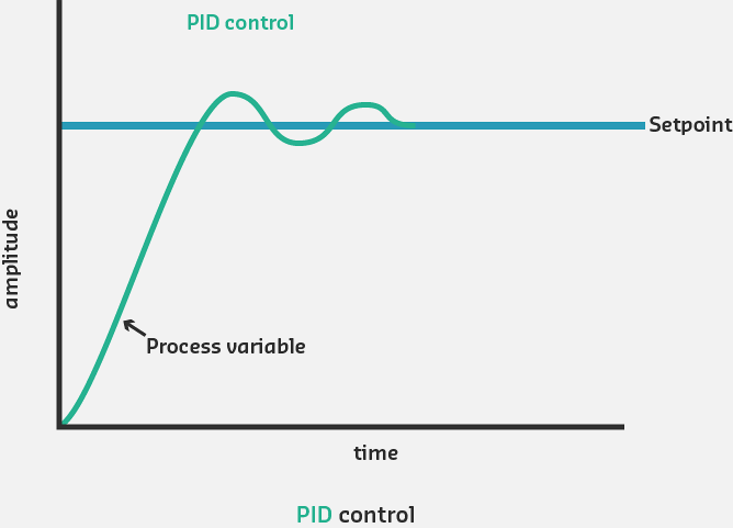
233  Integral and Derivative Control

233.1 Learning Objectives

By the end of this chapter, you will be able to:

  • Explain how integral control eliminates steady-state error
  • Identify and mitigate integral windup problems
  • Describe how derivative control reduces overshoot and provides damping
  • Compare P-only, PI, and PID control configurations
  • Select the appropriate PID configuration for different applications

233.2 Integral Control (I)
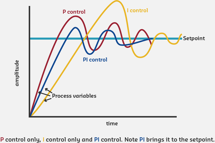
Diagram showing integral control addition to system with error signal being accumulated over time through integration, multiplied by integral gain Ki to produce output that grows continuously until error reaches zero, eliminating persistent steady-state offset that proportional control alone cannot fix
Figure 233.1: Diagram showing addition of integral control action to eliminate steady-state error by accumulating error over time

The Integral term accumulates error over time and provides control action based on the total accumulated error. This eliminates steady-state error that P-only control cannot handle.

\[ u_i(t) = K_i \cdot \int_{0}^{t} e(\tau) \, d\tau \]

%%{init: {'theme': 'base', 'themeVariables': { 'primaryColor': '#2C3E50', 'primaryTextColor': '#fff', 'primaryBorderColor': '#16A085', 'lineColor': '#16A085', 'secondaryColor': '#E67E22', 'tertiaryColor': '#ecf0f1', 'fontSize': '15px'}}}%%
graph TB
    Error["Error<br/>e(t)"] -->|Accumulate<br/>Over Time| Int["Integral<br/>∫e(t) dt"]
    Int -->|Multiply by Ki| Gain["Integral<br/>Gain<br/>Ki"]
    Gain -->|Output = Ki × ∫e dt| Output["Control<br/>Output<br/>u_i(t)"]

    Persist["Persistent<br/>Small Error<br/>e = 0.5°C"] -.->|"Accumulates:<br/>0.5+0.5+0.5..."| Growing["Growing<br/>Integral<br/>Output"]
    Growing -.->|"Increases Until<br/>Error = 0"| Zero["Zero<br/>Steady-State<br/>Error"]

    style Error fill:#E67E22,stroke:#16A085,stroke-width:2px,color:#fff
    style Int fill:#2C3E50,stroke:#16A085,stroke-width:2px,color:#fff
    style Gain fill:#2C3E50,stroke:#16A085,stroke-width:2px,color:#fff
    style Output fill:#16A085,stroke:#2C3E50,stroke-width:2px,color:#fff
    style Zero fill:#16A085,stroke:#2C3E50,stroke-width:3px,color:#fff

Figure 233.2: Integral: accumulates error until steady-state offset eliminated

Integral Control Mechanism: Accumulates error over time. Even small persistent errors grow the integral, increasing control output until error reaches exactly zero. Eliminates steady-state offset that P-only cannot fix.

How Integral Control Works:

  • Accumulates error over time: \(\int e(t) dt\)
  • If error persists (even small error), integral grows
  • Integral keeps increasing until error becomes zero
  • Also called “automatic reset” - resets bias until error eliminated
TipAnalogy: Lane Change with Crosswind (Need for Integral)

Continuing the driving analogy, now add a crosswind (disturbance):

%%{init: {'theme': 'base', 'themeVariables': { 'primaryColor': '#2C3E50', 'primaryTextColor': '#fff', 'primaryBorderColor': '#16A085', 'lineColor': '#16A085', 'secondaryColor': '#E67E22', 'tertiaryColor': '#ecf0f1', 'fontSize': '14px'}}}%%
graph TB
    subgraph POnly ["P-Only Control + Crosswind"]
        P1["Target Lane<br/>Center"] --> P2["P Term<br/>Steers Toward<br/>Target"]
        P2 --> P3["Car Approaches"]
        Wind1["Crosswind<br/>Pushes Car<br/>Right"] -.->|Constant Force| P3
        P3 --> P4["Settles Left<br/>of Center<br/>(Steady-State<br/>Error)"]
    end

    subgraph PI ["PI Control + Crosswind"]
        I1["Target Lane<br/>Center"] --> I2["P Term<br/>Initial Steering"]
        I2 --> I3["Crosswind<br/>Creates Error"]
        I3 --> I4["I Term<br/>Accumulates<br/>Error"]
        I4 --> I5["Increases<br/>Steering<br/>Over Time"]
        I5 --> I6["Reaches<br/>Exact Center<br/>(Zero Error)"]
    end

    style P4 fill:#E74C3C,stroke:#2C3E50,stroke-width:2px,color:#fff
    style I6 fill:#16A085,stroke:#2C3E50,stroke-width:3px,color:#fff

Figure 233.3: P-only vs PI: integral eliminates crosswind-caused offset

Integral Term Necessity with Disturbances: P-only control settles with offset when constant disturbance (crosswind) opposes control action. Integral term accumulates persistent error and increases output until exactly compensating for disturbance, achieving zero steady-state error.

P-Only Response to Crosswind: - Initial steering (Kp times error) moves car toward target - Crosswind counteracts steering - Car settles with persistent offset (steady-state error) - Driver maintains constant steering, but never reaches center

PI Response to Crosswind: - P term provides initial response (Kp times error) - Crosswind creates persistent error - I term accumulates this error over time - Integral output increases until steering overcomes crosswind - Car reaches exact center of lane - Error becomes zero, integral stops growing

Mathematical Intuition:

The integral accumulates (sums) all past errors:

Time | Error | Proportional | Integral Accumulated | Total Output
-----|-------|-------------|---------------------|-------------
0s   | +3C   | Kp×3 = 1.5  | 0                   | 1.5
1s   | +2C   | Kp×2 = 1.0  | Ki×(3+2) = 0.5      | 1.5
2s   | +1C   | Kp×1 = 0.5  | Ki×(3+2+1) = 0.6    | 1.1
3s   | +1C   | Kp×1 = 0.5  | Ki×(3+2+1+1) = 0.7  | 1.2
4s   | 0C    | Kp×0 = 0    | Ki×(3+2+1+1+0) = 0.7| 0.7
5s   | 0C    | Kp×0 = 0    | Ki×(3+2+1+1+0+0)=0.7| 0.7

Kp = 0.5, Ki = 0.1

Key Observations: - Even when P term drops to zero (error = 0), I term maintains output - This compensates for disturbances requiring sustained control action - Integral prevents steady-state error

Benefits of Adding Integral:

  1. Eliminates steady-state error: System reaches exact set point
  2. Compensates for disturbances: Overcomes constant external forces
  3. Automatic adjustment: No manual reset needed

Cautions with Integral:

  1. Integral Windup: Integral can accumulate excessively during large errors
  2. Slower Response: Can slow down initial response
  3. Overshoot: Can cause overshoot if Ki too large
  4. Requires Careful Tuning: Ki must be chosen carefully
WarningIntegral Windup Problem

If a large error persists for a long time (e.g., system startup, actuator saturation), the integral can accumulate to very large values. This is called integral windup.

Consequences: - When error finally reverses, huge accumulated integral causes massive overshoot - System may oscillate wildly or become unstable

Solutions: - Limit integral accumulation (clamping) - Reset integral when actuator saturates - Anti-windup algorithms in modern controllers

Question: Integral windup occurs when a controller’s integral term accumulates excessively. When is this most problematic?

Explanation: Integral windup scenario: Cold room (10C) to Setpoint 22C leads to large error. Heater maxes at 100% but temperature slowly rises. Error persists so integral keeps accumulating massive value. Finally reaches 22C but integral is huge so heater stays at 100% even above setpoint causing severe overshoot to 28C. Solution: Anti-windup mechanisms: 1) Clamping - stop integrating when output saturated, 2) Back-calculation - reduce integral when saturating, 3) Conditional integration - only integrate when actuator not saturated. Real example: Oven preheating - without anti-windup, overshoots 50C past target. With anti-windup, smooth approach.

Question: A water tank level controller has steady-state error - the level stabilizes at 95cm instead of the 100cm setpoint. Which PID term eliminates this?

Explanation: Steady-state error occurs when P-only control equilibrates below setpoint. At 95cm, small error (5cm) produces small output, insufficient to reach 100cm but enough to prevent dropping further. Integral term solves this: Accumulates error over time: 5cm times 60s = 300 cm-s accumulated error. Ki times 300 gives increased output that pushes toward setpoint. Process: Even tiny persistent error eventually creates large integral term forcing correction. Real example: Room stabilizes at 21.5C instead of 22C so Integral accumulates 0.5C error for minutes leading to increased heater output and reaching 22C. Integral eliminates offset but can cause overshoot if too aggressive.

233.3 Derivative Control (D)

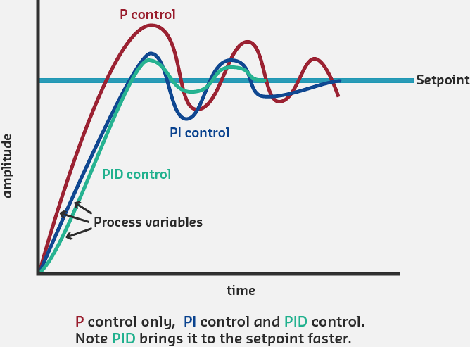
Diagram showing derivative control addition to system with error rate of change being calculated, multiplied by derivative gain Kd to produce damping output that opposes rapid changes, reducing overshoot by providing predictive braking action when system approaches setpoint quickly, preventing oscillation
Figure 233.4: Diagram showing addition of derivative control action to reduce overshoot and improve stability by responding to rate of error change

The Derivative term provides control action based on the rate of change of error. It anticipates future error trends and provides damping to prevent overshoot.

\[ u_d(t) = K_d \cdot \frac{de(t)}{dt} \]

%%{init: {'theme': 'base', 'themeVariables': { 'primaryColor': '#2C3E50', 'primaryTextColor': '#fff', 'primaryBorderColor': '#16A085', 'lineColor': '#16A085', 'secondaryColor': '#E67E22', 'tertiaryColor': '#ecf0f1', 'fontSize': '15px'}}}%%
graph TB
    Error["Error<br/>e(t)"] -->|Calculate Rate<br/>of Change| Deriv["Derivative<br/>de(t)/dt"]
    Deriv -->|Multiply by Kd| Gain["Derivative<br/>Gain<br/>Kd"]
    Gain -->|Output = Kd × de/dt| Output["Control<br/>Output<br/>u_d(t)"]

    Fast["Error Decreasing<br/>Rapidly<br/>de/dt = -2°C/s"] -.->|Negative<br/>Derivative| Brake["Negative Output<br/>(Reduce Control)<br/>Prevents Overshoot"]
    Slow["Error Stable<br/>de/dt = 0"] -.->|Zero<br/>Derivative| None["No D<br/>Contribution"]

    style Error fill:#E67E22,stroke:#16A085,stroke-width:2px,color:#fff
    style Deriv fill:#2C3E50,stroke:#16A085,stroke-width:2px,color:#fff
    style Gain fill:#2C3E50,stroke:#16A085,stroke-width:2px,color:#fff
    style Output fill:#16A085,stroke:#2C3E50,stroke-width:2px,color:#fff
    style Brake fill:#16A085,stroke:#2C3E50,stroke-width:3px,color:#fff

Figure 233.5: Derivative: rate of change provides predictive braking

Derivative Control Mechanism: Measures rate of error change. Rapid error decrease (approaching target fast) produces negative D output, reducing control action preemptively to prevent overshoot. Acts as predictive damping brake.

How Derivative Control Works:

  • Measures how fast error is changing: \(\frac{de}{dt}\)
  • If error decreasing rapidly, derivative is negative
  • Negative derivative reduces control action (anticipates reaching target)
  • Provides damping effect to prevent overshoot
  • Acts as predictive brake
TipAnalogy: High-Speed Lane Change (Need for Derivative)

Now consider changing lanes at high speed where momentum causes overshoot:

%%{init: {'theme': 'base', 'themeVariables': { 'primaryColor': '#2C3E50', 'primaryTextColor': '#fff', 'primaryBorderColor': '#16A085', 'lineColor': '#16A085', 'secondaryColor': '#E67E22', 'tertiaryColor': '#ecf0f1', 'fontSize': '14px'}}}%%
graph TB
    subgraph PIOnly ["PI Control (No D) - High Speed Lane Change"]
        PI1["Large Error"] --> PI2["Strong P+I<br/>Steering"]
        PI2 --> PI3["Car Accelerates<br/>Toward Target"]
        PI3 --> PI4["Momentum<br/>Carries Past<br/>(Overshoot)"]
        PI4 --> PI5["Oscillates<br/>Back and Forth"]
        PI5 -.->|Multiple<br/>Corrections| PI4
    end

    subgraph PID ["PID Control (With D) - High Speed Lane Change"]
        D1["Large Error"] --> D2["Strong P+I<br/>Steering"]
        D2 --> D3["As Approaching:<br/>Error Decreasing<br/>Rapidly"]
        D3 --> D4["D Term<br/>Detects<br/>de/dt < 0"]
        D4 --> D5["Reduces<br/>Steering<br/>Preemptively"]
        D5 --> D6["Smooth Arrival<br/>No Overshoot"]
    end

    style PI4 fill:#E74C3C,stroke:#2C3E50,stroke-width:2px,color:#fff
    style PI5 fill:#E74C3C,stroke:#2C3E50,stroke-width:2px,color:#fff
    style D6 fill:#16A085,stroke:#2C3E50,stroke-width:3px,color:#fff

Figure 233.6: PI vs PID: derivative prevents high-speed overshoot

Derivative Term Prevents Overshoot: PI control without D term overshoots at high speed due to momentum, causing oscillation. PID control’s D term detects rapid approach (large negative de/dt), reduces control action preemptively, achieving smooth arrival without overshoot.

Without Derivative (PI only at high speed): 1. Large error leads to strong steering (P + I) 2. Car accelerates toward target lane 3. Momentum carries car past target (overshoot) 4. Must steer back (oscillation) 5. May oscillate several times before settling

With Derivative (PID at high speed): 1. Large error leads to strong steering (P + I + D) 2. As car approaches target, error decreases rapidly 3. Derivative detects rapid error change: \(\frac{de}{dt} < 0\) 4. Derivative produces negative output, reducing total control 5. Steering reduced proportionally to approach speed 6. Car smoothly reaches target without overshoot

Derivative Calculation Example:

Time | Error | Error Change | P Output | I Output | D Output | Total
-----|-------|--------------|----------|----------|----------|------
0s   | +5C   | —            | 2.5      | 0        | 0        | 2.5
1s   | +4C   | -1C/s        | 2.0      | 0.45     | -0.3     | 2.15
2s   | +2C   | -2C/s        | 1.0      | 0.55     | -0.6     | 0.95
3s   | +0.5C | -1.5C/s      | 0.25     | 0.6      | -0.45    | 0.4
4s   | 0C    | -0.5C/s      | 0        | 0.6      | -0.15    | 0.45
5s   | 0C    | 0C/s         | 0        | 0.6      | 0        | 0.6

Kp = 0.5, Ki = 0.05, Kd = 0.3
Error Change = (Current Error - Previous Error) / Δt

Key Observations: - When error decreases rapidly (large negative de/dt), D term is negative - Negative D term reduces total output, slowing approach - As approach slows (de/dt approaches 0), D term reduces to zero - D acts as damping, preventing overshoot from P and I

Benefits of Adding Derivative:

  1. Reduces overshoot: Dampens aggressive P and I responses
  2. Improves stability: Prevents oscillations
  3. Faster settling: Reaches steady state more quickly
  4. Better response to changing conditions: Anticipates trends

Cautions with Derivative:

  1. Noise sensitivity: Amplifies high-frequency noise in sensor readings
  2. Difficult to tune: Kd selection is challenging
  3. Rarely used alone: Almost always combined with P and/or I
  4. May prevent reaching target: Excessive Kd can slow response too much

233.4 PID Control Summary
Complete PID control system diagram showing setpoint and measured value feeding into error calculation, error splitting into three parallel control paths (proportional for present error, integral for accumulated past error, derivative for predicted future error), all three terms summing to produce optimal combined control output driving process plant
Figure 233.7: Complete PID control system showing all three control actions working together: P (immediate response), I (eliminates offset), D (reduces overshoot)

%%{init: {'theme': 'base', 'themeVariables': { 'primaryColor': '#2C3E50', 'primaryTextColor': '#fff', 'primaryBorderColor': '#16A085', 'lineColor': '#16A085', 'secondaryColor': '#E67E22', 'tertiaryColor': '#ecf0f1', 'fontSize': '15px'}}}%%
graph TB
    SP["Setpoint"] --> Comp["Error<br/>Calculation"]
    Meas["Measured<br/>Value"] --> Comp

    Comp -->|"e(t)"| P["P: Present<br/>Kp × e(t)<br/>Fast Response"]
    Comp -->|"∫e dt"| I["I: Past<br/>Ki × ∫e dt<br/>Eliminate Offset"]
    Comp -->|"de/dt"| D["D: Future<br/>Kd × de/dt<br/>Prevent Overshoot"]

    P --> Sum["Σ<br/>Combined<br/>Output"]
    I --> Sum
    D --> Sum

    Sum -->|"u(t) = P + I + D"| Plant["Process"]
    Plant --> Meas

    style Comp fill:#E67E22,stroke:#16A085,stroke-width:2px,color:#fff
    style P fill:#2C3E50,stroke:#16A085,stroke-width:2px,color:#fff
    style I fill:#2C3E50,stroke:#16A085,stroke-width:2px,color:#fff
    style D fill:#2C3E50,stroke:#16A085,stroke-width:2px,color:#fff
    style Sum fill:#16A085,stroke:#2C3E50,stroke-width:3px,color:#fff
    style Plant fill:#7F8C8D,stroke:#16A085,stroke-width:2px,color:#fff

Figure 233.8: Complete PID: P (present), I (past), D (future) combined

Complete PID Controller Architecture: Error drives three parallel control actions. P term addresses present error (fast), I term corrects accumulated past error (accuracy), D term anticipates future trends (stability). Combined output creates optimal control signal.

ImportantPID Term Summary
Term Reacts To Purpose Issue to Watch
P Current error magnitude Provide proportional response Steady-state error, overshoot
I Accumulated error over time Eliminate steady-state error Integral windup, slow response
D Rate of error change Dampen overshoot, predict future Noise amplification, hard to tune

Simplified Summary: - P corrects present error - I corrects past accumulated error - D corrects future predicted error

Response Comparison:

%%{init: {'theme': 'base', 'themeVariables': { 'primaryColor': '#2C3E50', 'primaryTextColor': '#fff', 'primaryBorderColor': '#16A085', 'lineColor': '#16A085', 'secondaryColor': '#E67E22', 'tertiaryColor': '#ecf0f1', 'fontSize': '14px'}}}%%
graph LR
    subgraph POnly ["P-Only"]
        P1["Fast<br/>Response"] --> P2["Steady-State<br/>Error<br/>Remains"]
    end

    subgraph PI ["PI Control"]
        I1["Good<br/>Response"] --> I2["Zero<br/>Steady-State<br/>Error"]
        I2 --> I3["Possible<br/>Overshoot"]
    end

    subgraph PID ["PID Control"]
        D1["Fast<br/>Response"] --> D2["Zero<br/>Steady-State<br/>Error"]
        D2 --> D3["Minimal<br/>Overshoot<br/>Best Performance"]
    end

    style P2 fill:#E74C3C,stroke:#2C3E50,stroke-width:2px,color:#fff
    style I3 fill:#E67E22,stroke:#16A085,stroke-width:2px,color:#fff
    style D3 fill:#16A085,stroke:#2C3E50,stroke-width:3px,color:#fff

Figure 233.9: P vs PI vs PID: performance trade-off comparison

PID Configuration Performance Comparison: P-only provides fast response but leaves steady-state error. PI eliminates error but may overshoot. Full PID combines fast response, zero error, and minimal overshoot for optimal performance.

When to Use Each Configuration:

  • P Only: Simple systems, fast response needed, some error acceptable
  • PI: Most common, general-purpose control, steady-state accuracy required
  • PID: High-performance applications, minimal overshoot critical
  • PD: Rare, fast servos with no steady-state error concerns
WarningCommon Misconception: “Higher Gains Always Mean Better Control”

The Myth: Many beginners believe that increasing all PID gains (Kp, Ki, Kd) will result in faster, more accurate control. Reality proves otherwise.

Real-World Example: A commercial smart greenhouse ventilation system experienced catastrophic oscillations after technicians “optimized” the temperature controller by doubling all PID gains.

What Happened: - Original tuning: Kp=2.0, Ki=0.5, Kd=1.0 led to smooth control, plus-minus 0.3C stability, 5-minute settling time - “Optimized” tuning: Kp=4.0, Ki=1.0, Kd=2.0 led to severe oscillations, plus-minus 4C swings, vent motors cycling every 30 seconds - Motor damage: $8,500 in burnt-out actuators from excessive cycling (12,000 cycles/day vs. rated 5,000 cycles/day) - Crop loss: $45,000 in heat-stressed tomato plants due to temperature instability

Why Aggressive Tuning Fails:

  1. Excessive Kp leads to overshoot and oscillation. Temperature overshoots target by 5-8C, system corrects aggressively in opposite direction, creating sustained oscillation.
  2. Excessive Ki leads to integral windup. During startup, integral accumulates massive value while system heats up slowly. When finally reaching setpoint, huge integral term causes 10C+ overshoot taking 30+ minutes to correct.
  3. Excessive Kd leads to noise amplification. Sensor noise (plus-minus 0.1C measurement variation) gets amplified by derivative term, causing actuator “chatter” - rapid on/off cycling that wears mechanical components.

The Truth About PID Tuning: - Balanced gains create stable control with acceptable response time - Conservative tuning (slightly slower) is more robust to disturbances and noise - Field conditions (sensor noise, actuator delays, thermal lag) limit achievable performance - Diminishing returns: Gains beyond optimal provide marginal speed improvement but dramatic stability degradation

Correct Approach: - Start with conservative gains (low values) - Gradually increase Kp until seeing slight overshoot - Add Ki slowly to eliminate steady-state error - Add minimal Kd only if overshoot remains problematic - Accept that 10-15% overshoot with 2-5 minute settling time is often optimal for real systems

Measured Impact (from greenhouse case study): - Reverting to original conservative tuning reduced motor cycling from 12,000 to 400 cycles/day (30x reduction) - Temperature stability improved from plus-minus 4C to plus-minus 0.3C (13x improvement) - System operated reliably for 3+ years with no further actuator failures

233.6 Summary

This chapter covered the Integral and Derivative components of PID control:

Key Takeaways:

  1. Integral Control (I): Accumulates error over time to eliminate steady-state error that P-only control cannot address

  2. Integral Windup: A dangerous condition where the integral accumulates excessively during prolonged errors - requires anti-windup mechanisms

  3. Derivative Control (D): Responds to the rate of error change, providing predictive braking to reduce overshoot

  4. D Term Limitations: Sensitive to sensor noise and difficult to tune - often omitted in favor of PI control

  5. Configuration Selection: PI is most common for general-purpose control; full PID only needed when minimal overshoot is critical

  6. Tuning Philosophy: Conservative, balanced gains outperform aggressive tuning in real-world conditions

233.7 What’s Next?

In the next chapter, we’ll explore hands-on PID implementation with labs, Arduino/ESP32 code examples, and production-ready frameworks.

Continue to PID Implementation and Labs