%%{init: {'theme': 'base', 'themeVariables': { 'primaryColor': '#2C3E50', 'primaryTextColor': '#fff', 'primaryBorderColor': '#16A085', 'lineColor': '#16A085', 'secondaryColor': '#E67E22', 'tertiaryColor': '#7F8C8D'}}}%%
graph TB
    DIO["DIO<br/>DODAG Information Object<br/>Advertise DODAG"]
    DIS["DIS<br/>DODAG Information Solicitation<br/>Request DODAG info"]
    DAO["DAO<br/>Destination Advertisement Object<br/>Advertise reachability"]
    DAOACK["DAO-ACK<br/>Acknowledge DAO"]

    ROOT["ROOT sends DIO"]
    NODE["Node receives DIO"]
    JOIN["Node joins DODAG"]
    ADV["Node sends DAO"]

    ROOT --> NODE
    NODE --> JOIN
    JOIN --> ADV

    style DIO fill:#2C3E50,stroke:#16A085,color:#fff,stroke-width:3px
    style DIS fill:#16A085,stroke:#2C3E50,color:#fff
    style DAO fill:#E67E22,stroke:#2C3E50,color:#fff
    style DAOACK fill:#7F8C8D,stroke:#2C3E50,color:#fff
    style ROOT fill:#2C3E50,stroke:#16A085,color:#fff
    style NODE fill:#16A085,stroke:#2C3E50,color:#fff
    style JOIN fill:#E67E22,stroke:#2C3E50,color:#fff
    style ADV fill:#7F8C8D,stroke:#2C3E50,color:#fff
707 RPL DODAG Construction and Routing Modes
NoteLearning Objectives
By the end of this section, you will be able to:
- Understand the step-by-step DODAG construction process
- Explain RPL control messages (DIO, DIS, DAO, DAO-ACK)
- Compare Storing mode vs Non-Storing mode in RPL
- Analyze memory and performance trade-offs between modes
- Choose the appropriate RPL mode for different deployment scenarios
707.1 Prerequisites
Before diving into this chapter, you should be familiar with:
- RPL Introduction and Core Concepts: Understanding DODAG topology, RANK mechanism, and why RPL is needed for IoT
- Routing Fundamentals: Knowledge of basic routing concepts and distance-vector protocols
NoteRelated Chapters
This Series: - RPL Introduction - Core concepts and fundamentals - RPL DODAG Construction and Modes - This chapter - RPL Traffic Patterns and Design - Traffic patterns and network design lab - RPL Production and Summary - Production framework and key takeaways
Hands-On: - RPL Production and Review - Storing vs Non-Storing mode deployment - Simulations Hub - Test RPL DODAG formation in simulators
707.2 DODAG Construction Process
RPL builds the DODAG through control messages:
{fig-alt=“RPL control messages overview showing DIO (advertise DODAG), DIS (request info), DAO (advertise reachability), DAO-ACK (acknowledgment), and DODAG construction flow from ROOT sending DIO through node joining to DAO advertisement”}
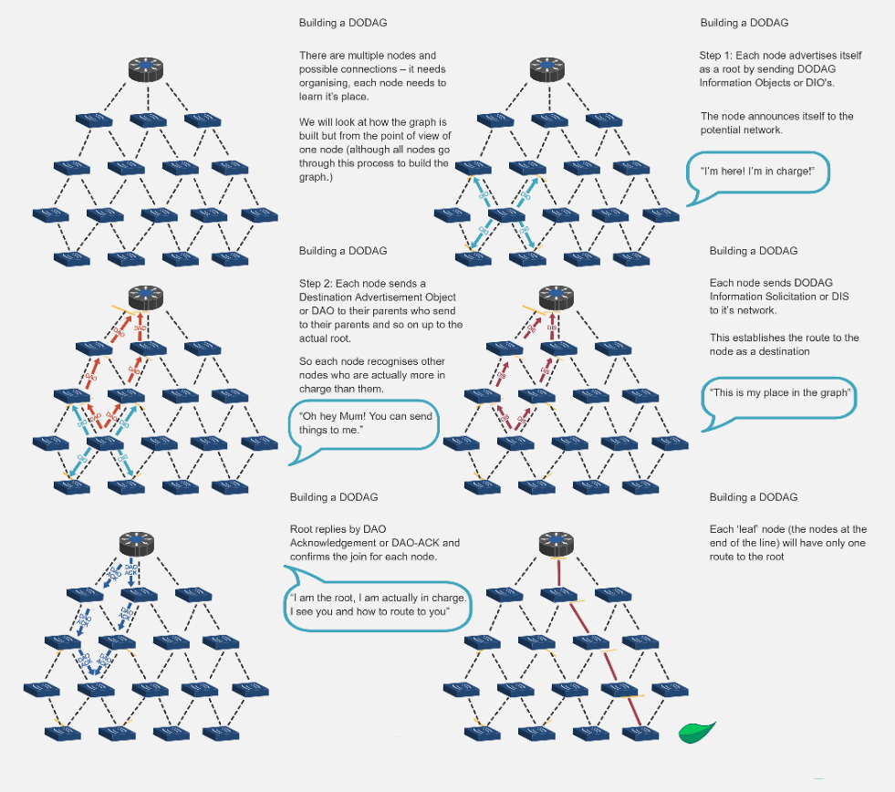
707.2.1 Step-by-Step DODAG Construction
%%{init: {'theme': 'base', 'themeVariables': { 'primaryColor': '#2C3E50', 'primaryTextColor': '#fff', 'primaryBorderColor': '#16A085', 'lineColor': '#16A085', 'secondaryColor': '#E67E22', 'tertiaryColor': '#7F8C8D'}}}%%
sequenceDiagram
    participant ROOT as ROOT (Rank 0)
    participant N1 as Node 1
    participant N2 as Node 2
    participant N3 as Node 3

    Note over ROOT: Step 1: ROOT initiates DODAG
    ROOT->>ROOT: Create DODAG ID<br/>Set RANK = 0
    ROOT->>N1: DIO (DODAG_ID, RANK=0)
    ROOT->>N2: DIO (DODAG_ID, RANK=0)

    Note over N1,N2: Step 2: Nodes receive DIO and join
    N1->>N1: Calculate RANK = 100<br/>Select ROOT as parent
    N2->>N2: Calculate RANK = 100<br/>Select ROOT as parent

    Note over N1,N2: Step 3: Nodes propagate DIO
    N1->>N3: DIO (DODAG_ID, RANK=100)
    N2->>N3: DIO (DODAG_ID, RANK=100)

    Note over N3: Step 4: Build upward routes
    N3->>N3: Calculate RANK = 200<br/>Select N1 as parent<br/>Parent pointer established

    Note over N3: Step 5: Build downward routes
    N3->>N1: DAO (I am reachable)
    N1->>ROOT: DAO (N3 reachable via me)
    ROOT->>N1: DAO-ACK
{fig-alt=“DODAG construction sequence diagram showing 5 steps: ROOT initiates with DIO, nodes receive and join calculating RANK, nodes propagate DIO, upward routes established via parent pointers, downward routes built via DAO messages”}
707.2.2 Detailed Construction Steps
NoteStep 1: Root Initiates DODAG
Root node (border router/gateway): 1. Creates DODAG: Assigns unique DODAG ID 2. Sets RANK = 0: Root has minimum RANK 3. Broadcasts DIO: Sends DODAG Information Object (multicast)
DIO Contents: - DODAG ID (IPv6 address) - RANK (0 for root) - Objective function (routing metric) - DODAG configuration (timers, etc.)
707.3 Step 2: Nodes Receive DIO and Join
Node receives DIO: 1. Decision: Join this DODAG or wait for others? - Compare DODAG rank, objective function - May receive DIOs from multiple DODAGs 2. Calculate RANK: RANK = parent_RANK + increase 3. Select parent: Choose sender of DIO (if acceptable) 4. Update state: Store DODAG ID, parent, RANK
Multiple DIO Sources: - Node may hear DIOs from multiple neighbors - Chooses best parent (lowest RANK, best link quality) - May maintain backup parents (loop-free)
707.4 Step 3: Nodes Propagate DIO
After joining DODAG: 1. Node becomes part of DODAG 2. Sends own DIO: Advertises DODAG to neighbors 3. DIO contents: Own RANK, DODAG ID, etc. 4. Trickle timer: Controls DIO frequency (adaptive)
Trickle Algorithm: - Stable network: Send DIOs infrequently (minutes) - Network changes: Send DIOs frequently (seconds) - Reduces overhead while maintaining responsiveness
NoteStep 4: Build Upward Routes
Upward routes (towards root) established automatically: - Each node knows its parent (from DIO selection) - Default route: Send to parent (towards root) - No routing table needed for upward routes (just parent pointer)
Example:
Node 3 -> Node 1 -> Root
(N3 knows parent is N1, N1 knows parent is Root)
NoteStep 5: Build Downward Routes (Storing Mode)
Downward routes (from root to nodes) require DAO messages:
- Node sends DAO to parent:
- “I am reachable via you”
- Includes node’s address and prefixes
- Parent updates routing table:
- “Node X is reachable via this child”
- Parent propagates DAO towards root:
- Aggregates reachability information
- Root knows all nodes:
- Complete routing table for downward routes
DAO-ACK (optional): - Parent confirms DAO receipt - Reliability for critical networks
707.5 RPL Routing Modes
RPL supports two modes with different memory/performance trade-offs:
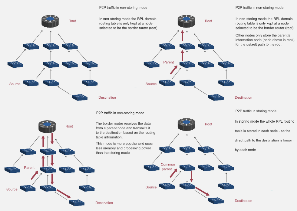
707.5.1 Storing Mode
Each node maintains routing table for its sub-DODAG.
%%{init: {'theme': 'base', 'themeVariables': { 'primaryColor': '#2C3E50', 'primaryTextColor': '#fff', 'primaryBorderColor': '#16A085', 'lineColor': '#16A085', 'secondaryColor': '#E67E22', 'tertiaryColor': '#7F8C8D'}}}%%
graph TB
    A["ROOT A<br/>Rank: 0<br/>Routing Table:<br/>B->B, C->B, D->C<br/>E->B, F->B"]
    B["Node B<br/>Rank: 100<br/>Routing Table:<br/>E->E, F->F"]
    C["Node C<br/>Rank: 100<br/>Routing Table:<br/>D->D"]
    D["Node D<br/>Rank: 200"]
    E["Node E<br/>Rank: 200"]
    F["Node F<br/>Rank: 200"]

    A --> B
    A --> C
    B --> E
    B --> F
    C --> D

    style A fill:#2C3E50,stroke:#16A085,color:#fff,stroke-width:3px
    style B fill:#16A085,stroke:#2C3E50,color:#fff
    style C fill:#16A085,stroke:#2C3E50,color:#fff
    style D fill:#E67E22,stroke:#2C3E50,color:#fff
    style E fill:#E67E22,stroke:#2C3E50,color:#fff
    style F fill:#E67E22,stroke:#2C3E50,color:#fff
{fig-alt=“RPL Storing mode showing distributed routing tables: ROOT maintains routes to all nodes, intermediate nodes B and C maintain routes to their descendants, enabling distributed forwarding decisions”}
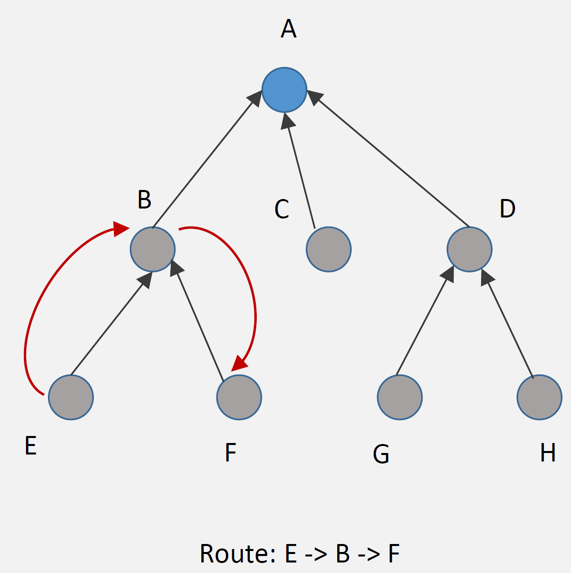
How It Works: 1. DAO messages: Nodes advertise reachability to parents 2. Routing tables: Each node stores routes to descendants 3. Packet forwarding: Node looks up destination in table, forwards to appropriate child
Example Route (E to F):
Step 1: E sends packet to parent B (upward)
Step 2: B checks routing table: "F is my child"
Step 3: B forwards directly to F (downward)

Route: E -> B -> F (optimal)Advantages: - Efficient routing: Optimal paths (no detour through root) - Low latency: Direct routes between any nodes - Root not bottleneck: Distributed routing decisions
Disadvantages: - Memory overhead: Each node stores routing table - Scalability: Routing tables grow with network size - Updates: DAO messages for every node change
Best For: - Devices with sufficient memory (32+ KB RAM) - Networks requiring low latency - Point-to-point communication common
707.5.2 Non-Storing Mode
Only root maintains routing information; exploits source routing.
%%{init: {'theme': 'base', 'themeVariables': { 'primaryColor': '#2C3E50', 'primaryTextColor': '#fff', 'primaryBorderColor': '#16A085', 'lineColor': '#16A085', 'secondaryColor': '#E67E22', 'tertiaryColor': '#7F8C8D'}}}%%
graph TB
    A["ROOT A<br/>Rank: 0<br/>Routing Table:<br/>B->B, C->C, D->C,D<br/>E->B,E, F->B,F<br/>(Complete topology)"]
    B["Node B<br/>Rank: 100<br/>Parent pointer only<br/>(No routing table)"]
    C["Node C<br/>Rank: 100<br/>Parent pointer only<br/>(No routing table)"]
    D["Node D<br/>Rank: 200<br/>Parent: C"]
    E["Node E<br/>Rank: 200<br/>Parent: B"]
    F["Node F<br/>Rank: 200<br/>Parent: B"]

    A --> B
    A --> C
    B --> E
    B --> F
    C --> D

    style A fill:#2C3E50,stroke:#16A085,color:#fff,stroke-width:3px
    style B fill:#16A085,stroke:#2C3E50,color:#fff
    style C fill:#16A085,stroke:#2C3E50,color:#fff
    style D fill:#7F8C8D,stroke:#2C3E50,color:#fff
    style E fill:#7F8C8D,stroke:#2C3E50,color:#fff
    style F fill:#7F8C8D,stroke:#2C3E50,color:#fff
{fig-alt=“RPL Non-Storing mode showing centralized routing at ROOT with complete topology, intermediate nodes maintain only parent pointers, downward routing uses source routing headers from root”}
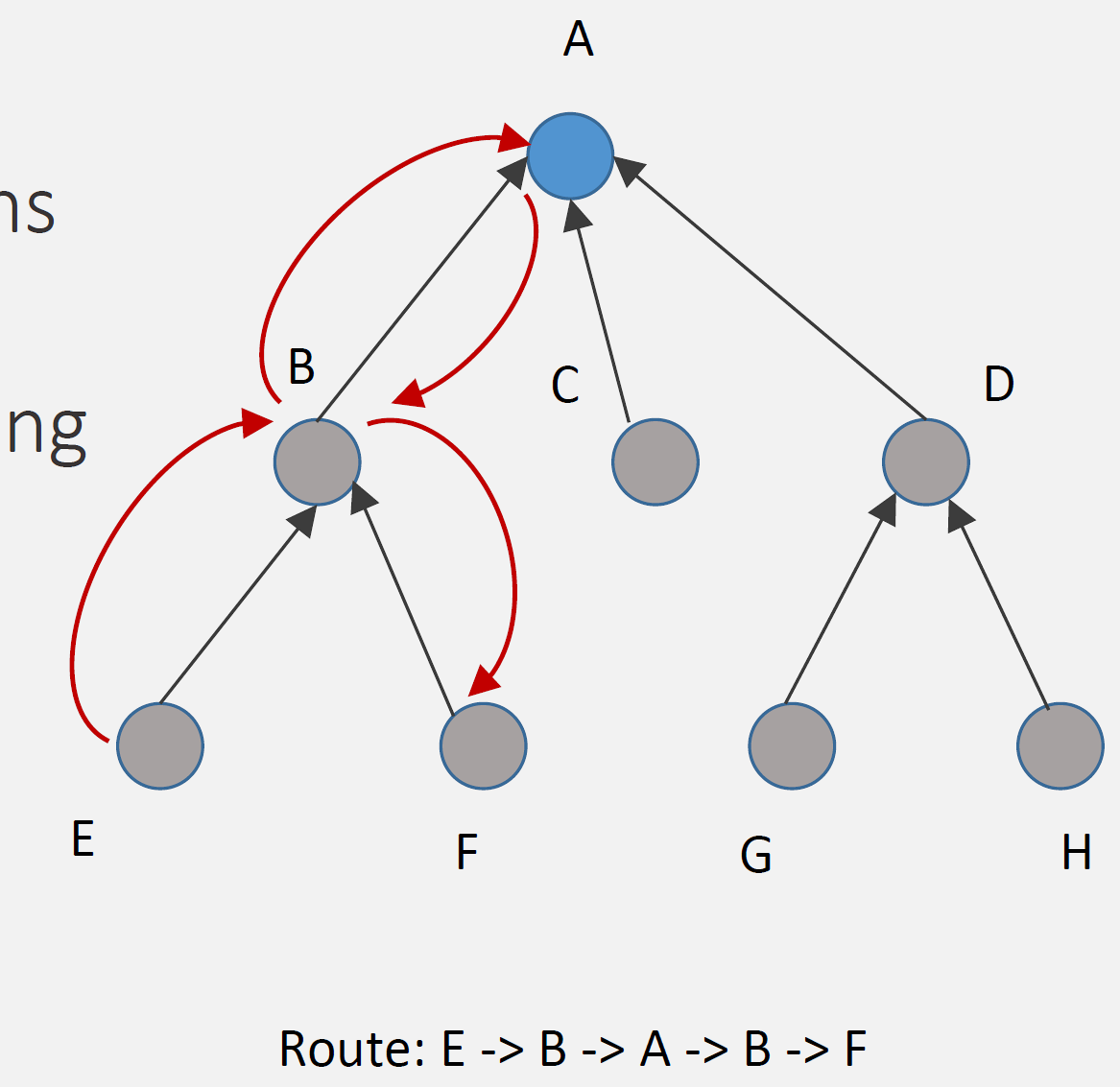
How It Works: 1. DAO to root: All nodes send DAO directly to root (upward) 2. Root stores all routes: Only root has complete routing table 3. Source routing: Root inserts complete path in packet header 4. Nodes forward: Follow instructions in packet header (no table lookup)
Example Route (E to F):
Step 1: E sends packet to parent B (upward, default route)
Step 2: B forwards to parent A (root) (upward, default route)
Step 3: A (root) checks routing table: "F via B"
Step 4: A inserts source route: [B, F]
Step 5: A sends to B with route in header
Step 6: B forwards to F following route

Route: E -> B -> A -> B -> F (via root)Advantages: - Low memory: Nodes don’t store routing tables (just parent) - Simple nodes: Minimal routing logic - Scalability: Network size doesn’t affect node memory
Disadvantages: - Suboptimal routes: All point-to-point traffic via root - Higher latency: Extra hops through root - Root bottleneck: All routing decisions at root - Header overhead: Source route in every packet
Best For: - Resource-constrained devices (< 16 KB RAM) - Primarily many-to-one traffic (sensors to gateway) - Point-to-point communication rare - Large networks (many nodes)
707.5.3 Storing vs Non-Storing Comparison
| Aspect | Storing Mode | Non-Storing Mode |
|---|---|---|
| Routing Table | Distributed (all nodes) | Centralized (root only) |
| Node Memory | Higher (routing table) | Lower (parent pointer only) |
| Route Optimality | Optimal (direct paths) | Suboptimal (via root) |
| Latency | Lower | Higher (extra hops) |
| Root Load | Low | High (all routing decisions) |
| Scalability | Limited by node memory | Limited by root capacity |
| DAO Destination | Parent | Root (through parents) |
| Header Overhead | Low | High (source routing) |
| Best For | Powerful nodes, low latency | Constrained nodes, many-to-one |
TipAlternative View: RPL Mode Selection Decision Tree
This variant provides a practical decision guide for choosing between Storing and Non-Storing modes based on your network characteristics.
%%{init: {'theme': 'base', 'themeVariables': {'primaryColor': '#2C3E50', 'primaryTextColor': '#fff', 'primaryBorderColor': '#16A085', 'lineColor': '#E67E22', 'secondaryColor': '#16A085', 'tertiaryColor': '#E8F6F3', 'fontSize': '10px'}}}%%
flowchart TD
    START["RPL Mode<br/>Selection"] --> Q1{"Primary traffic<br/>pattern?"}

    Q1 -->|"Many-to-One<br/>(sensors to gateway)"| Q2{"Node memory<br/>available?"}
    Q1 -->|"Point-to-Point<br/>(device to device)"| Q3{"Latency<br/>requirement?"}

    Q2 -->|"< 64KB RAM"| NS1["NON-STORING<br/>Memory efficient<br/>Root handles routing<br/>Best: Sensor networks"]
    Q2 -->|"> 64KB RAM"| Q4{"Network size?"}

    Q3 -->|"< 100ms"| ST1["STORING<br/>Direct P2P routes<br/>Lower latency<br/>Best: Industrial control"]
    Q3 -->|"> 100ms OK"| NS2["NON-STORING"]

    Q4 -->|"< 200 nodes"| ST2["STORING<br/>Optimal paths<br/>Distributed load<br/>Best: Building automation"]
    Q4 -->|"> 200 nodes"| NS3["NON-STORING<br/>Scales better<br/>Root manages all"]

    style START fill:#2C3E50,stroke:#16A085,color:#fff
    style Q1 fill:#16A085,stroke:#2C3E50,color:#fff
    style Q2 fill:#16A085,stroke:#2C3E50,color:#fff
    style Q3 fill:#16A085,stroke:#2C3E50,color:#fff
    style Q4 fill:#16A085,stroke:#2C3E50,color:#fff
    style NS1 fill:#E67E22,stroke:#2C3E50,color:#fff
    style NS2 fill:#E67E22,stroke:#2C3E50,color:#fff
    style NS3 fill:#E67E22,stroke:#2C3E50,color:#fff
    style ST1 fill:#2C3E50,stroke:#16A085,color:#fff
    style ST2 fill:#2C3E50,stroke:#16A085,color:#fff
Key Insight: Non-Storing mode is the default choice for resource-constrained sensor networks. Only move to Storing mode when you have both the memory budget AND specific P2P or latency requirements.
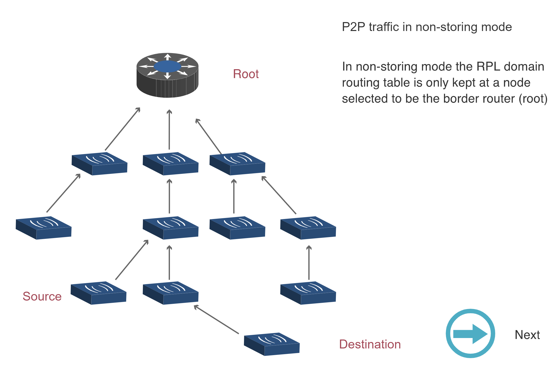
NoteAcademic Reference: P2P Traffic Routing Sequence
The following sequence diagrams illustrate how RPL handles point-to-point (P2P) traffic in Non-Storing and Storing modes.
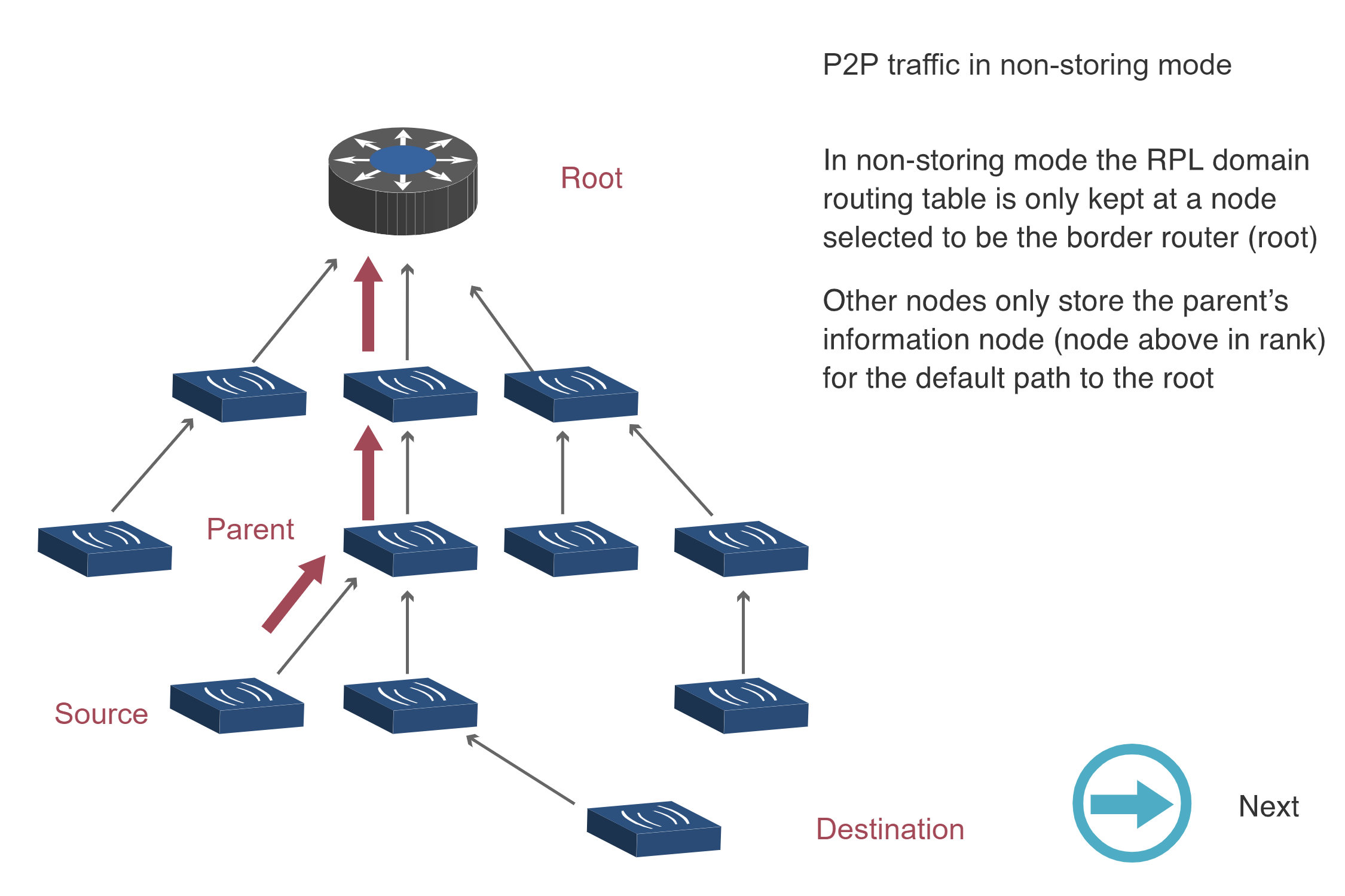
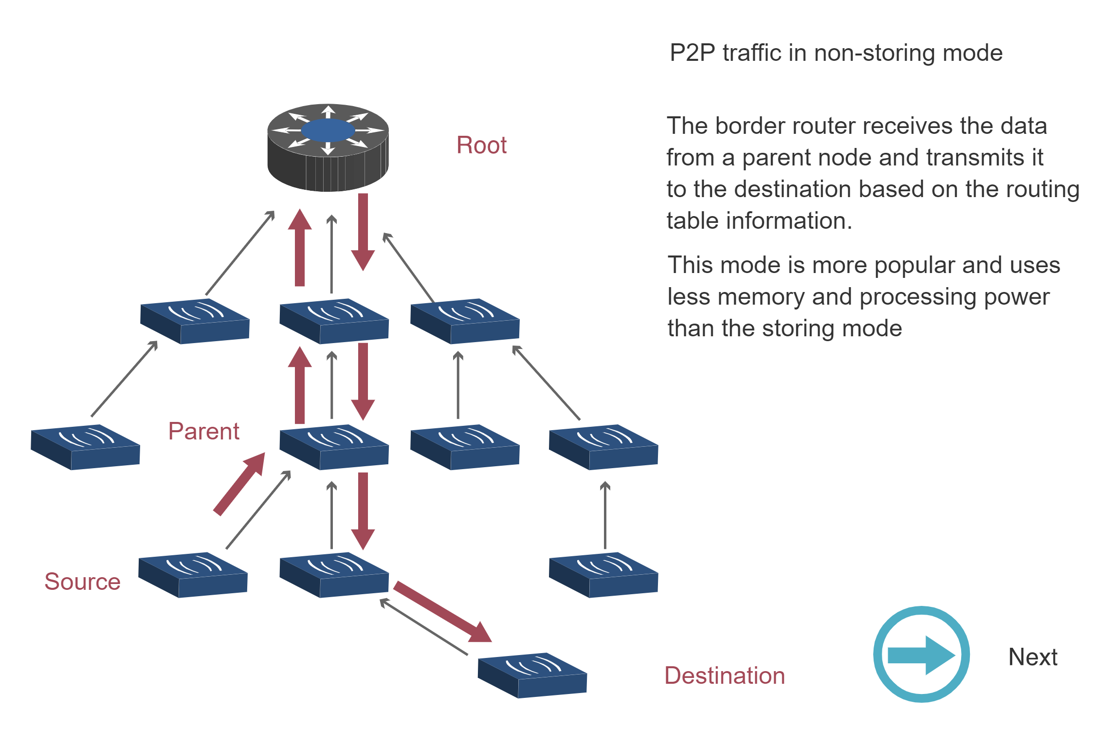
Non-Storing Mode P2P Traffic (Steps 1-3):
Storing Mode P2P Traffic:
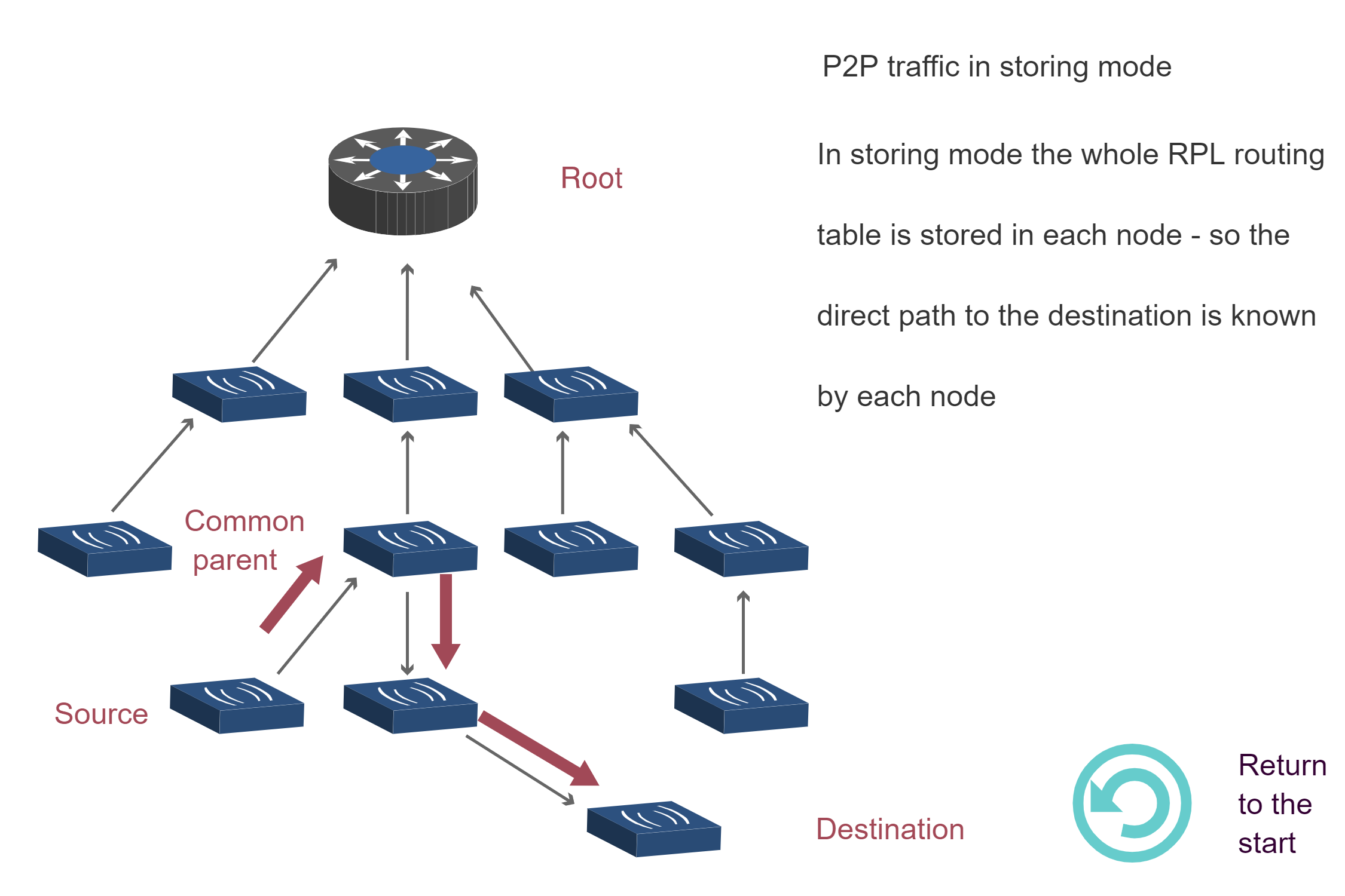
Key Insight: Non-Storing mode requires all P2P traffic to traverse the root (3 diagrams showing upward then downward path), while Storing mode enables direct routing through the nearest common ancestor (1 diagram showing optimized path). This explains why Storing mode has lower latency for P2P traffic despite higher memory requirements.
Source: CP IoT System Design Guide, Chapter 4 - Routing
707.6 What’s Next
Now that you understand how RPL constructs DODAGs and the trade-offs between Storing and Non-Storing modes, the next chapter covers traffic patterns and hands-on network design.
Continue to: RPL Traffic Patterns and Design
- Many-to-one, one-to-many, and point-to-point traffic patterns
- Hands-on lab: Designing RPL network for smart building
- Memory requirements calculation
- Traffic pattern analysis and mode selection