713 RPL Summary and Interactive Tools

713.1 Common Pitfalls

Common Pitfalls

1. Choosing the Wrong RPL Mode (Storing vs Non-Storing)

Mistake: Using Storing mode on severely memory-constrained nodes (e.g., 2KB RAM sensors), causing routing table overflow and network instability when nodes cannot store routes to all descendants
Why it happens: Storing mode provides more efficient point-to-point routing, so developers default to it without calculating memory requirements. Each routing entry requires ~20-40 bytes; a node with 50 descendants needs 1-2KB just for routing tables
Solution: Calculate your network’s memory budget before choosing modes. Use Non-Storing mode when: (1) nodes have <8KB RAM, (2) network depth exceeds 4-5 hops, or (3) point-to-point traffic is rare. In Non-Storing mode, all downward routes go through the root, which must have sufficient memory but leaf nodes stay lightweight. For hybrid needs, consider using Storing mode only for nodes with adequate memory

2. Aggressive Trickle Timer Settings Causing Network Storms

Mistake: Setting Trickle timer Imin too low (e.g., 100ms) or Imax too small (e.g., 4 doublings) in dense networks, causing constant DIO flooding that overwhelms the radio channel and drains batteries
Why it happens: Developers test with small networks (3-5 nodes) where aggressive timers converge quickly. In production deployments with 50+ nodes, the same settings cause every node to transmit DIOs simultaneously during network events
Solution: Start with conservative Trickle settings: Imin = 2-4 seconds, Imax = 16-20 doublings (giving maximum intervals of hours). For stable networks, RPL naturally reduces DIO frequency through Trickle’s exponential backoff. Only decrease timers if convergence time is unacceptable for your application. Monitor DIO message rates - if you see >1 DIO/minute/node in steady state, your Trickle parameters are too aggressive

3. Single DODAG Root Without Redundancy

Mistake: Deploying production RPL networks with only one border router as the DODAG root, creating a single point of failure where root failure disconnects the entire network from the Internet
Why it happens: RPL documentation focuses on single-root DODAGs for simplicity. Adding multiple roots requires understanding RPL instances, DODAG IDs, and root coordination, which adds deployment complexity
Solution: For production deployments, configure multiple border routers with the same DODAG ID but different root preferences. Use RPL’s multiple DODAG instance feature to provide backup paths. Alternatively, deploy redundant roots with different DODAG IDs and configure important nodes to join both. Monitor root health and implement automatic failover scripts that promote a secondary root if the primary becomes unreachable

713.2 Summary

Distance-Vector Protocol: RPL is designed specifically for Low-Power and Lossy Networks (LLNs), using parent pointers and RANK values rather than complex link-state databases
DODAG Topology: Destination Oriented Directed Acyclic Graph structure with single root enables loop-free routing and efficient many-to-one traffic patterns
RANK Mechanism: Hierarchical position values prevent routing loops by enforcing that packets flow only toward lower RANK (toward root), calculated using objective functions
Control Messages: DIO (DODAG Information Object) advertises network, DIS (DODAG Information Solicitation) requests information, DAO (Destination Advertisement Object) builds downward routes
Routing Modes: Storing mode distributes routing tables across nodes for optimal paths, while Non-Storing mode centralizes routing at root to minimize node memory requirements
Traffic Optimization: Upward routing (many-to-one) uses minimal state with parent pointers, downward and point-to-point routing leverages mode-specific mechanisms
IoT-Specific Design: Trickle timer algorithm, ETX metrics, and support for multiple instances address resource constraints and lossy wireless links

Interactive: RPL DODAG Builder

Build and visualize an RPL DODAG (Destination Oriented Directed Acyclic Graph) interactively. Watch how nodes join the network, calculate their RANK based on different objective functions, and see DIO messages propagate through the tree.

Instructions:

Click “Add Node” to add new nodes to the network
Select different Objective Functions to see how RANK calculation changes
Watch how each node selects its parent based on the objective function
Observe the DIO propagation from root outward
Use “Reset Network” to start fresh

Show code

viewof objectiveFunction = Inputs.select(
  ["hop_count", "etx", "energy"],
  {
    value: "hop_count",
    label: "Objective Function",
    format: x => x === "hop_count" ? "Hop Count (OF0 - simple)" :
                 x === "etx" ? "ETX (Expected Transmission Count)" :
                 "Energy (minimize power consumption)"
  }
)

Show code

initialRoot = [{id: 0, name: "ROOT", x: 400, y: 50, rank: 0, parent: null, isRoot: true, etx: 1.0, energy: 100}]

mutable dodagNodes = initialRoot

mutable nodeCounter = 1

mutable messageLog = ["Network initialized. ROOT node created at RANK 0."]

Show code

function createNode(nodes, of, counter) {
  const layer = Math.floor(nodes.length / 3) + 1
  const nodesInLayer = nodes.filter(n => Math.floor(n.rank / 256) === layer - 1).length
  const xOffset = (nodesInLayer % 3 - 1) * 150
  const newX = Math.max(50, Math.min(750, 400 + xOffset + (Math.random() - 0.5) * 80))
  const newY = Math.max(100, Math.min(450, 50 + layer * 100 + (Math.random() - 0.5) * 30))

  const etxVal = 1.0 + Math.random() * 2.0
  const energyCost = 50 + Math.random() * 100

  let bestParent = null
  let bestCost = Infinity

  for (const p of nodes.filter(n => n.rank < 65535)) {
    const dist = Math.sqrt(Math.pow(newX - p.x, 2) + Math.pow(newY - p.y, 2))
    if (dist > 250) continue

    let cost = p.rank + 256
    if (of === "etx") cost = p.rank + Math.floor(etxVal * 256)
    else if (of === "energy") cost = p.rank + Math.floor(energyCost * 2)

    if (cost < bestCost) {
      bestCost = cost
      bestParent = p
    }
  }

  if (!bestParent) {
    bestParent = nodes.reduce((a, b) => {
      const distA = Math.sqrt(Math.pow(newX - a.x, 2) + Math.pow(newY - a.y, 2))
      const distB = Math.sqrt(Math.pow(newX - b.x, 2) + Math.pow(newY - b.y, 2))
      return distA < distB ? a : b
    })
    bestCost = bestParent.rank + 256
    if (of === "etx") bestCost = bestParent.rank + Math.floor(etxVal * 256)
    else if (of === "energy") bestCost = bestParent.rank + Math.floor(energyCost * 2)
  }

  return {
    id: counter,
    name: "Node " + String.fromCharCode(65 + counter - 1),
    x: newX,
    y: newY,
    rank: bestCost,
    parent: bestParent.id,
    parentName: bestParent.name,
    isRoot: false,
    etx: etxVal,
    energy: energyCost
  }
}

Show code

viewof addNodeBtn = Inputs.button("Add Node", {
  reduce: () => {
    if (dodagNodes.length >= 15) {
      mutable messageLog = [...messageLog.slice(-9), "Maximum 15 nodes reached. Reset to add more."]
      return
    }
    const newNode = createNode(dodagNodes, objectiveFunction, nodeCounter)
    mutable dodagNodes = [...dodagNodes, newNode]
    mutable nodeCounter = nodeCounter + 1
    const ofLabel = objectiveFunction === "hop_count" ? "Hop Count" :
                    objectiveFunction === "etx" ? "ETX" : "Energy"
    mutable messageLog = [...messageLog.slice(-9),
      "DIO received: " + newNode.name + " joined. Parent: " + newNode.parentName + ", RANK: " + newNode.rank + " (" + ofLabel + ")"
    ]
  }
})

viewof resetBtn = Inputs.button("Reset Network", {
  reduce: () => {
    mutable dodagNodes = initialRoot
    mutable nodeCounter = 1
    mutable messageLog = ["Network reset. ROOT node created at RANK 0."]
  }
})

Show code

dodagVisualization = {
  const width = 800
  const height = 500

  const svg = d3.create("svg")
    .attr("viewBox", [0, 0, width, height])
    .attr("width", "100%")
    .attr("height", height)
    .style("background", "#f8f9fa")
    .style("border-radius", "8px")
    .style("border", "1px solid #dee2e6")

  svg.append("text")
    .attr("x", width / 2)
    .attr("y", 25)
    .attr("text-anchor", "middle")
    .attr("font-size", "14px")
    .attr("font-weight", "bold")
    .attr("fill", "#2C3E50")
    .text("RPL DODAG Visualization")

  const edges = dodagNodes.filter(n => n.parent !== null)

  svg.selectAll("line.edge")
    .data(edges)
    .join("line")
    .attr("class", "edge")
    .attr("x1", d => dodagNodes.find(n => n.id === d.parent).x)
    .attr("y1", d => dodagNodes.find(n => n.id === d.parent).y)
    .attr("x2", d => d.x)
    .attr("y2", d => d.y)
    .attr("stroke", "#16A085")
    .attr("stroke-width", 2)
    .attr("stroke-dasharray", d => d.id === dodagNodes[dodagNodes.length - 1].id && dodagNodes.length > 1 ? "5,5" : "none")
    .attr("opacity", d => d.id === dodagNodes[dodagNodes.length - 1].id && dodagNodes.length > 1 ? 0.7 : 1)

  if (dodagNodes.length > 1) {
    const newest = dodagNodes[dodagNodes.length - 1]
    const parent = dodagNodes.find(n => n.id === newest.parent)
    if (parent) {
      const pulse = svg.append("circle")
        .attr("cx", parent.x)
        .attr("cy", parent.y)
        .attr("r", 5)
        .attr("fill", "#E67E22")
        .attr("opacity", 0.8)
      pulse.append("animate")
        .attr("attributeName", "r")
        .attr("from", 5)
        .attr("to", 30)
        .attr("dur", "1s")
        .attr("repeatCount", "3")
      pulse.append("animate")
        .attr("attributeName", "opacity")
        .attr("from", 0.8)
        .attr("to", 0)
        .attr("dur", "1s")
        .attr("repeatCount", "3")
    }
  }

  const nodeGroups = svg.selectAll("g.node")
    .data(dodagNodes)
    .join("g")
    .attr("class", "node")
    .attr("transform", d => "translate(" + d.x + ", " + d.y + ")")

  nodeGroups.append("circle")
    .attr("r", d => d.isRoot ? 25 : 20)
    .attr("fill", d => d.isRoot ? "#2C3E50" :
      d.id === dodagNodes[dodagNodes.length - 1].id && dodagNodes.length > 1 ? "#E67E22" : "#16A085")
    .attr("stroke", d => d.isRoot ? "#16A085" : "#2C3E50")
    .attr("stroke-width", d => d.isRoot ? 3 : 2)

  nodeGroups.append("text")
    .attr("text-anchor", "middle")
    .attr("dy", -30)
    .attr("font-size", "12px")
    .attr("font-weight", "bold")
    .attr("fill", "#2C3E50")
    .text(d => d.name)

  nodeGroups.append("text")
    .attr("text-anchor", "middle")
    .attr("dy", 5)
    .attr("font-size", "10px")
    .attr("fill", "white")
    .attr("font-weight", "bold")
    .text(d => d.rank)

  nodeGroups.append("text")
    .attr("text-anchor", "middle")
    .attr("dy", 35)
    .attr("font-size", "9px")
    .attr("fill", "#7F8C8D")
    .text(d => "RANK: " + d.rank)

  const legend = svg.append("g")
    .attr("transform", "translate(20, " + (height - 100) + ")")

  legend.append("rect")
    .attr("width", 180)
    .attr("height", 90)
    .attr("fill", "white")
    .attr("stroke", "#dee2e6")
    .attr("rx", 4)

  legend.append("text").attr("x", 10).attr("y", 18)
    .attr("font-size", "11px").attr("font-weight", "bold").attr("fill", "#2C3E50")
    .text("Legend:")

  legend.append("circle").attr("cx", 20).attr("cy", 38).attr("r", 8)
    .attr("fill", "#2C3E50").attr("stroke", "#16A085").attr("stroke-width", 2)
  legend.append("text").attr("x", 35).attr("y", 42)
    .attr("font-size", "10px").attr("fill", "#2C3E50").text("ROOT (RANK 0)")

  legend.append("circle").attr("cx", 20).attr("cy", 58).attr("r", 8).attr("fill", "#16A085")
  legend.append("text").attr("x", 35).attr("y", 62)
    .attr("font-size", "10px").attr("fill", "#2C3E50").text("Joined Node")

  legend.append("circle").attr("cx", 20).attr("cy", 78).attr("r", 8).attr("fill", "#E67E22")
  legend.append("text").attr("x", 35).attr("y", 82)
    .attr("font-size", "10px").attr("fill", "#2C3E50").text("Just Joined (DIO pulse)")

  const stats = svg.append("g")
    .attr("transform", "translate(" + (width - 200) + ", " + (height - 100) + ")")

  stats.append("rect").attr("width", 180).attr("height", 90)
    .attr("fill", "white").attr("stroke", "#dee2e6").attr("rx", 4)

  stats.append("text").attr("x", 10).attr("y", 18)
    .attr("font-size", "11px").attr("font-weight", "bold").attr("fill", "#2C3E50")
    .text("Network Stats:")

  stats.append("text").attr("x", 10).attr("y", 38)
    .attr("font-size", "10px").attr("fill", "#2C3E50")
    .text("Nodes: " + dodagNodes.length)

  const maxRank = Math.max(...dodagNodes.map(n => n.rank))
  const maxDepth = Math.ceil(maxRank / 256)

  stats.append("text").attr("x", 10).attr("y", 54)
    .attr("font-size", "10px").attr("fill", "#2C3E50")
    .text("Max RANK: " + maxRank)

  stats.append("text").attr("x", 10).attr("y", 70)
    .attr("font-size", "10px").attr("fill", "#2C3E50")
    .text("Est. Depth: ~" + maxDepth + " hops")

  const ofName = objectiveFunction === "hop_count" ? "Hop Count" :
                 objectiveFunction === "etx" ? "ETX" : "Energy"
  stats.append("text").attr("x", 10).attr("y", 86)
    .attr("font-size", "10px").attr("fill", "#2C3E50")
    .text("OF: " + ofName)

  return svg.node()
}

Show code

messageLogDisplay = html`<div style="background: #2C3E50; color: #16A085; padding: 12px; border-radius: 4px; font-family: monospace; font-size: 11px; max-height: 150px; overflow-y: auto; margin-top: 10px;">
  <div style="color: #E67E22; font-weight: bold; margin-bottom: 8px;">DIO/DAO Message Log (Trickle Timer Active):</div>
  ${messageLog.map(msg => html`<div style="margin: 2px 0; color: ${msg.includes('DIO') ? '#16A085' : msg.includes('reset') ? '#E67E22' : '#fff'};">-> ${msg}</div>`)}
</div>`

Show code

trickleInfo = html`<div style="background: #f8f9fa; border: 1px solid #dee2e6; border-radius: 4px; padding: 12px; margin-top: 10px;">
  <div style="font-weight: bold; color: #2C3E50; margin-bottom: 8px;">Trickle Timer Concept:</div>
  <div style="font-size: 12px; color: #495057; line-height: 1.5;">
    <p>In real RPL networks, the <strong>Trickle Timer</strong> controls DIO message frequency:</p>
    <ul style="margin: 8px 0;">
      <li><strong>Stable network</strong>: DIOs sent infrequently (minutes) to save energy</li>
      <li><strong>Network change</strong>: Timer resets, DIOs sent frequently (seconds) for fast convergence</li>
      <li><strong>Suppression</strong>: If neighbors already sent consistent DIOs, skip own transmission</li>
    </ul>
    <p style="color: #16A085;"><strong>Current simulation</strong>: Each "Add Node" simulates receiving a DIO and joining the DODAG. The orange pulse shows DIO propagation from the parent.</p>
  </div>
</div>`

Objective Function Details:

Function	RANK Calculation	Best For
Hop Count (OF0)	Parent RANK + 256 per hop	Simple networks, equal link quality
ETX	Parent RANK + (ETX x 256)	Lossy networks, reliability focus
Energy	Parent RANK + (Energy x 2)	Battery-powered, lifetime optimization

Try This:

Add 5-6 nodes and observe the tree structure
Switch objective functions and reset - notice how the same nodes may select different parents
Watch the orange DIO pulse showing message propagation
Note how RANK increases as you move away from ROOT

713.3 Original Source Figures (Alternative Views)

The following figures from the CP IoT System Design Guide provide alternative visual representations of RPL concepts covered in this chapter.

DAG and DODAG Structures (Source Figure)

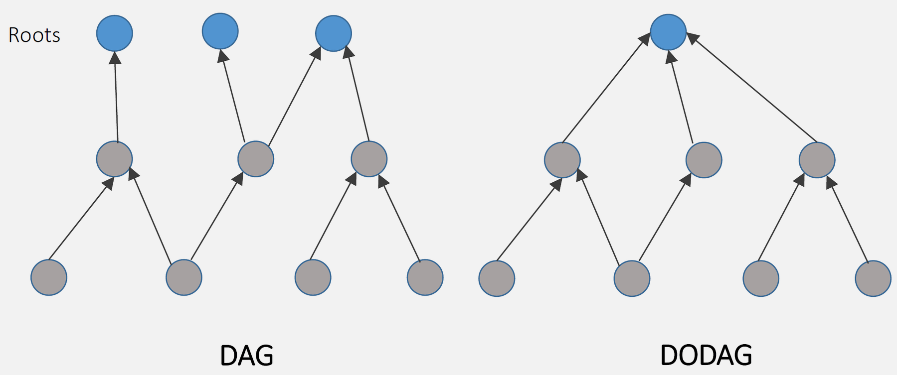
Original textbook figure showing the difference between a general Directed Acyclic Graph (DAG) with multiple roots and a DODAG (Destination-Oriented DAG) with a single root destination, illustrating how RPL creates tree-like structures for efficient IoT routing — DAG and DODAG comparison from original source

Source: CP IoT System Design Guide, Chapter 4 - Routing

RPL DAG and DODAG Formation Sequence

Step 1 of DODAG formation showing initial network state before RPL routing begins, with nodes scattered and no parent relationships established — RPL DAG and DODAG formation step 1

Step 2 of DODAG formation showing nodes beginning to receive DIO messages from the root and establishing initial parent selections — RPL DAG and DODAG formation step 2

Step 3 of DODAG formation showing complete tree structure with all nodes having selected preferred parents and routes to the root — RPL DAG and DODAG formation step 3

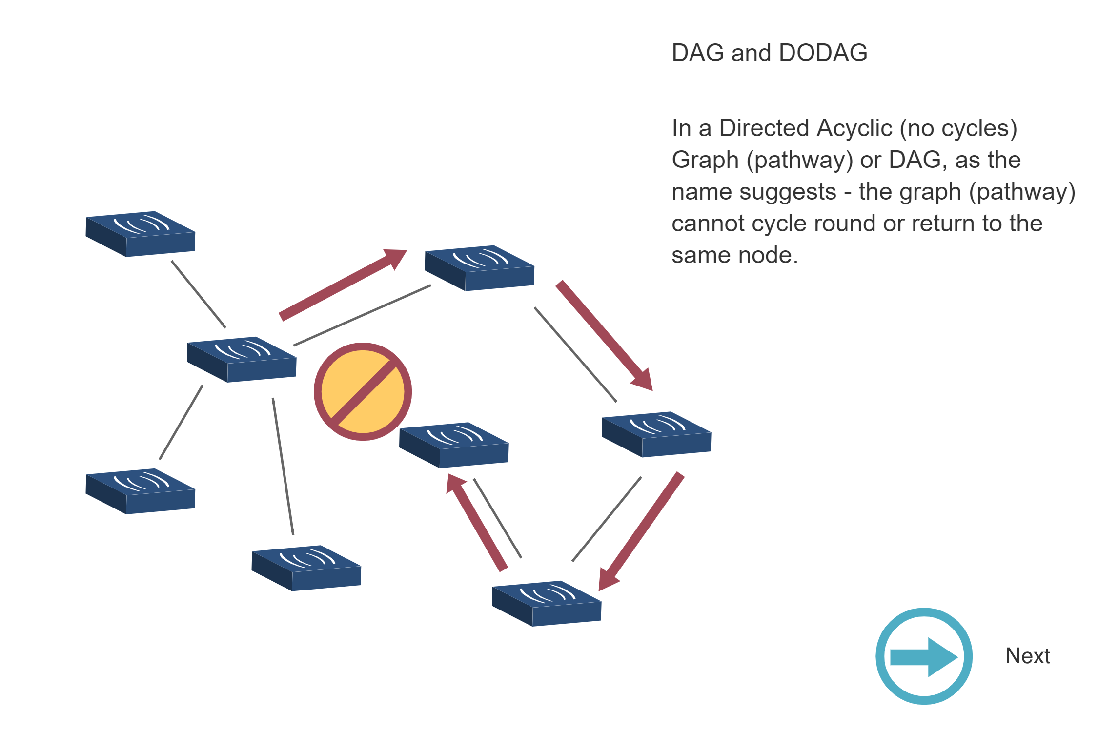
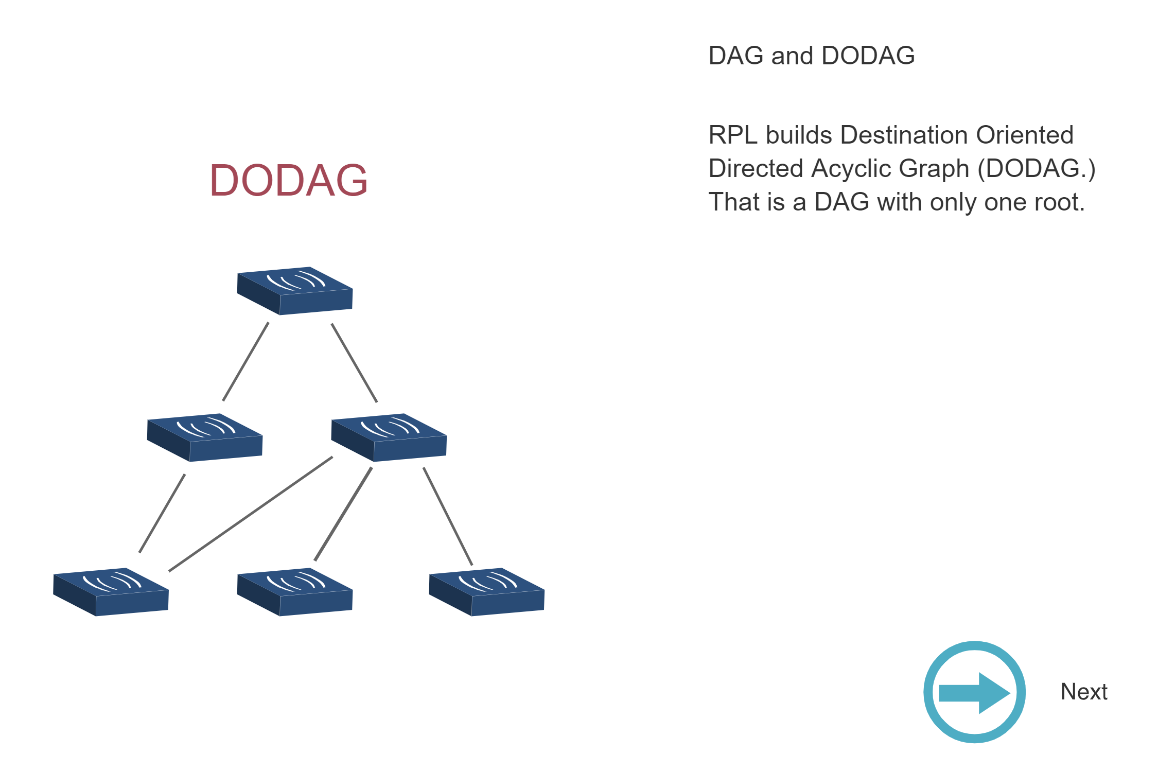
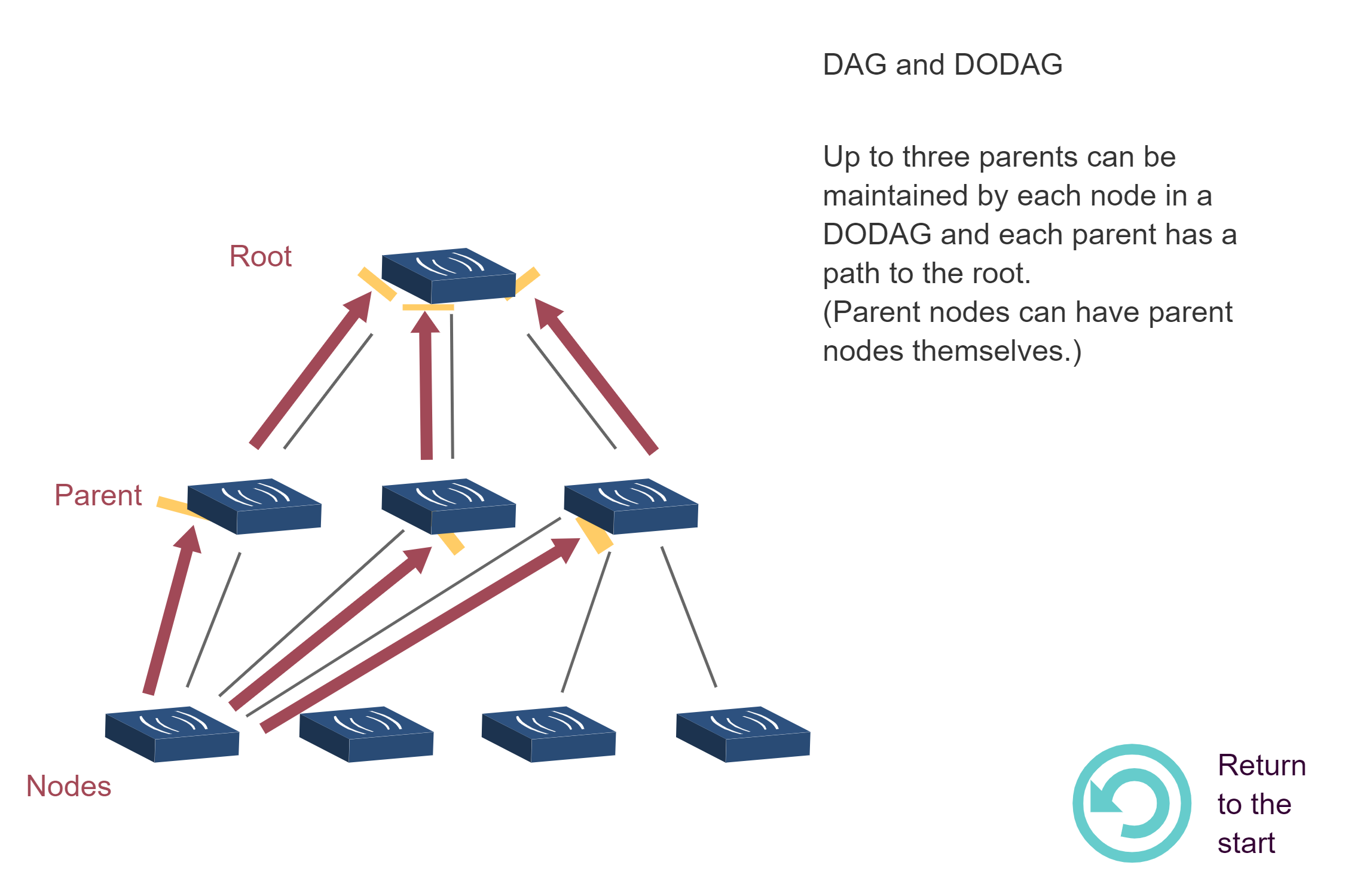
Source: CP IoT System Design Guide, Chapter 4 - Routing

RPL RANK Calculation Visualization

Complete visualization of RPL RANK values across a network showing how rank increases with distance from root, with root at rank 0 and leaf nodes at highest rank values — RPL Rank calculation overview

Step 1 of rank calculation showing root advertising rank 0 to immediate neighbors via DIO messages — RPL Rank step 1

Step 2 of rank calculation showing second-tier nodes calculating their rank based on parent rank plus link cost metric — RPL Rank step 2

Step 3 of rank calculation showing further propagation of rank values to deeper nodes in the network topology — RPL Rank step 3

Step 4 showing complete rank assignment across all nodes in the DODAG with final routing paths established — RPL Rank step 4

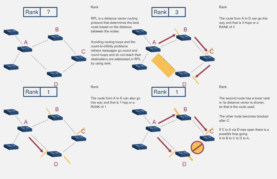
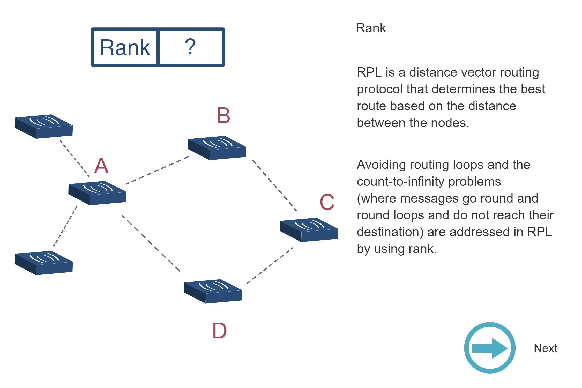
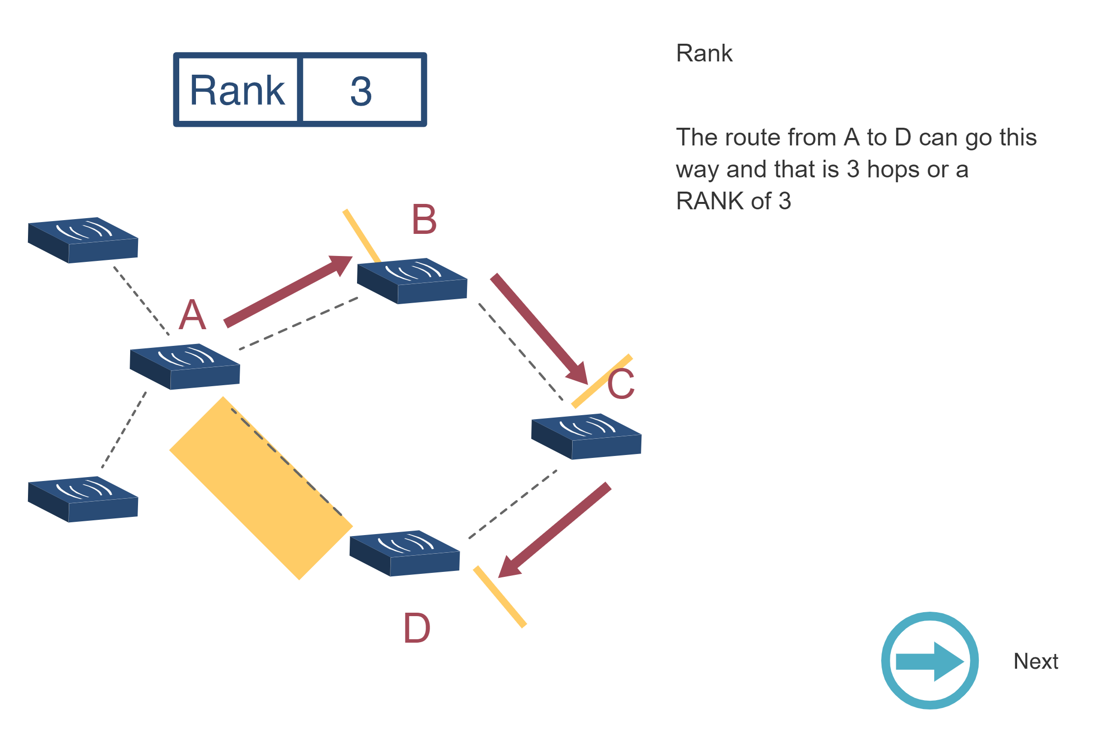
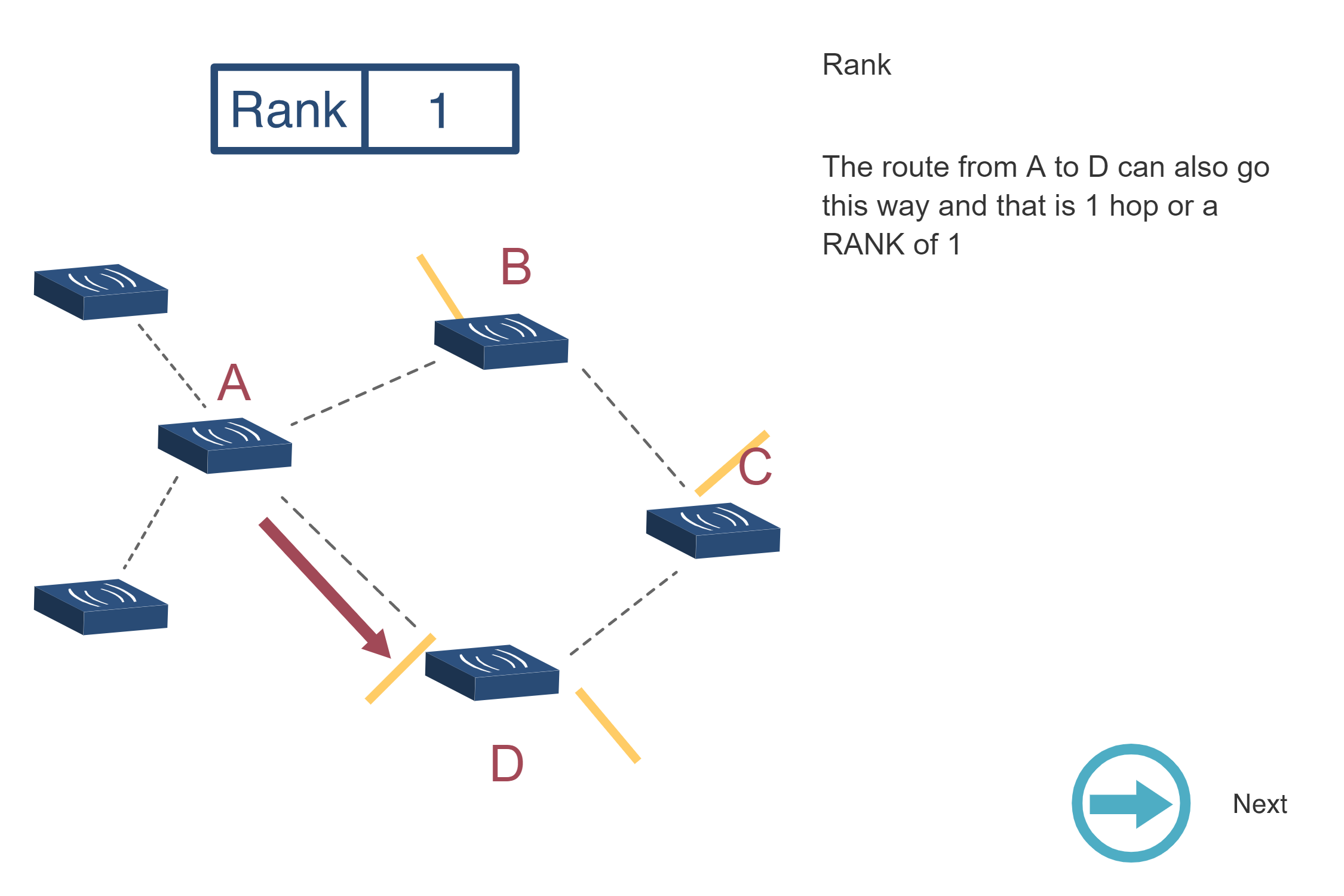
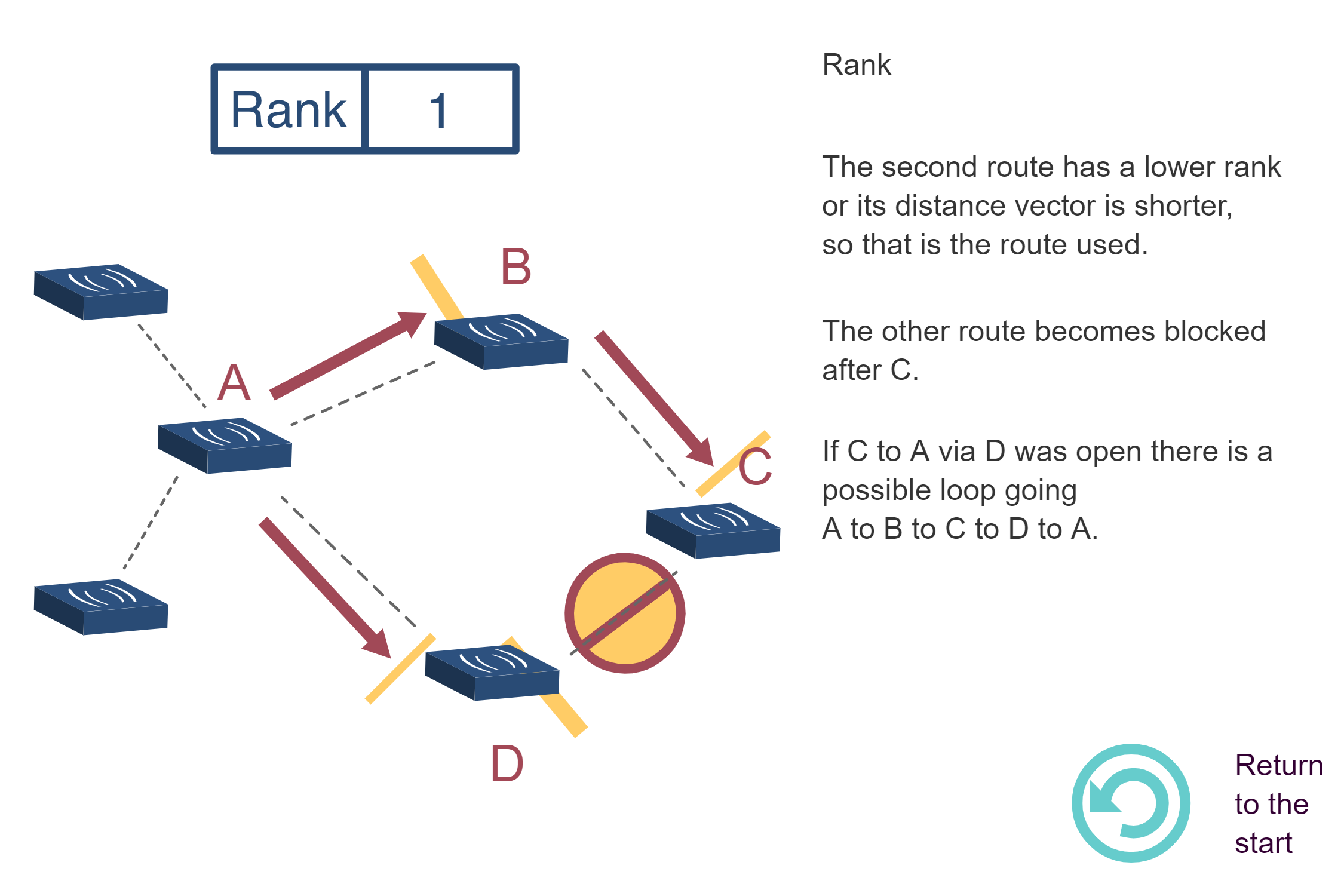
Source: CP IoT System Design Guide, Chapter 4 - Routing

Building a DODAG - Step-by-Step Process

Complete step-by-step visualization showing how a DODAG is constructed from initial state through final tree structure — Building a DODAG - Complete overview

DODAG building step 1: Root node initiates DODAG by sending first DIO message — Building a DODAG step 1

DODAG building step 2: Neighbors receive DIO, calculate rank, select root as parent — Building a DODAG step 2

DODAG building step 3: Second-tier nodes forward DIO messages to their neighbors — Building a DODAG step 3

DODAG building step 4: More nodes join DODAG, tree structure expands — Building a DODAG step 4

DODAG building step 5: Edge nodes receive DIO and select parents — Building a DODAG step 5

DODAG building step 6: Complete DODAG formed with all nodes having routes to root — Building a DODAG step 6

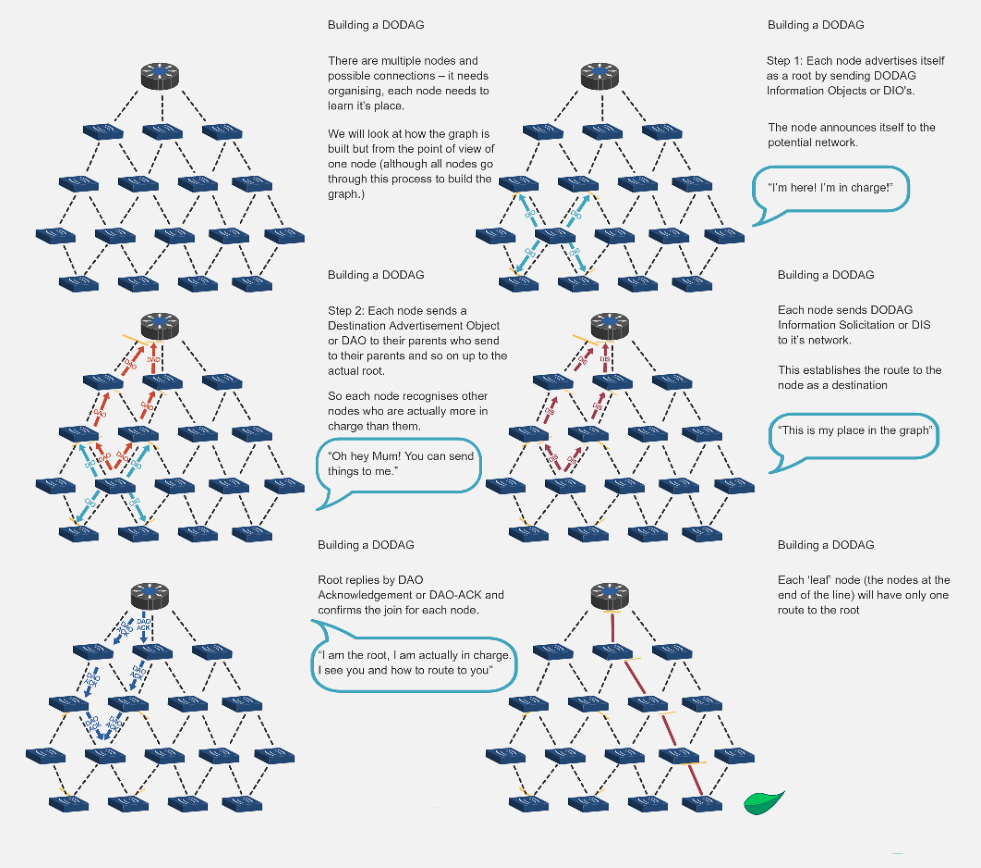
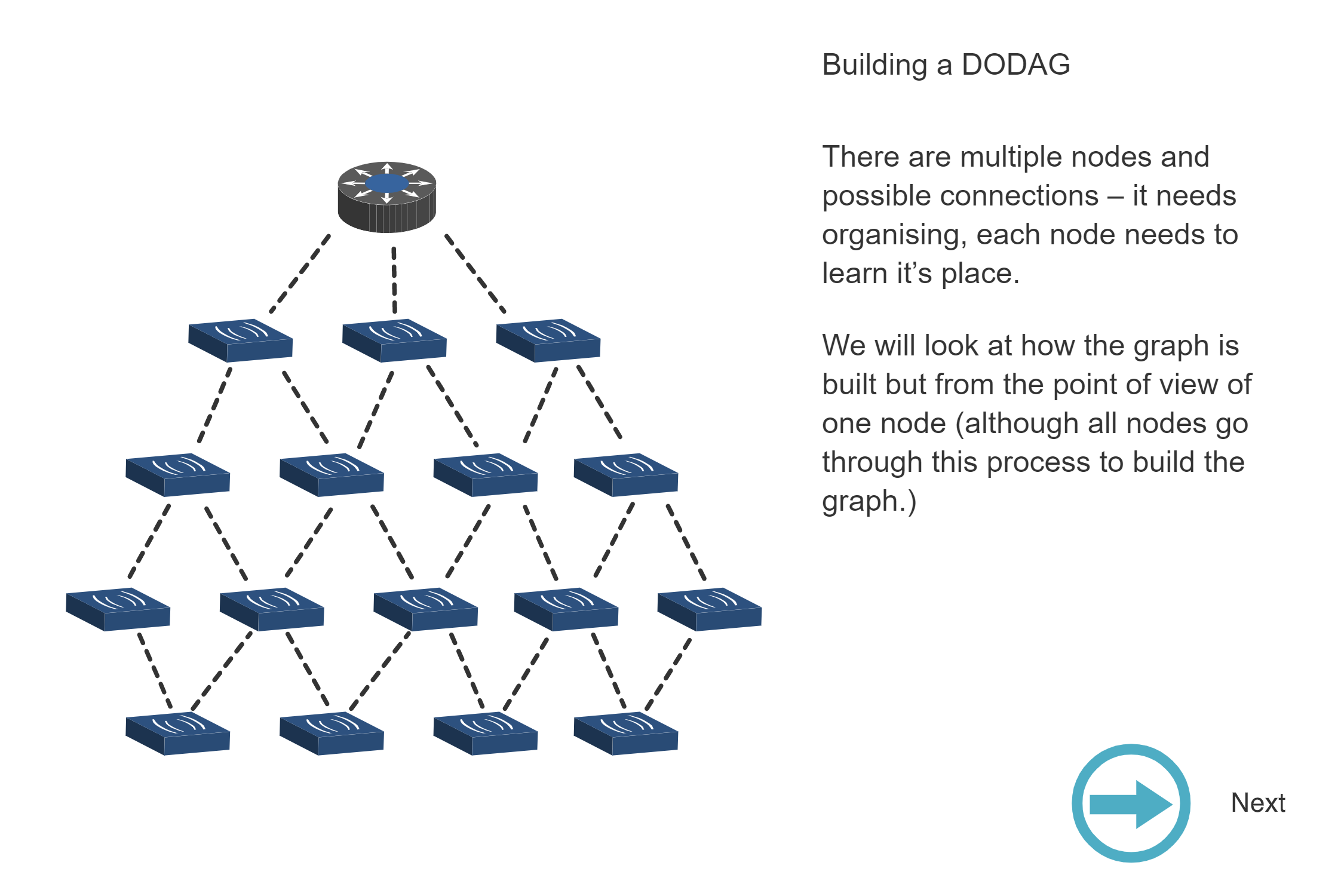
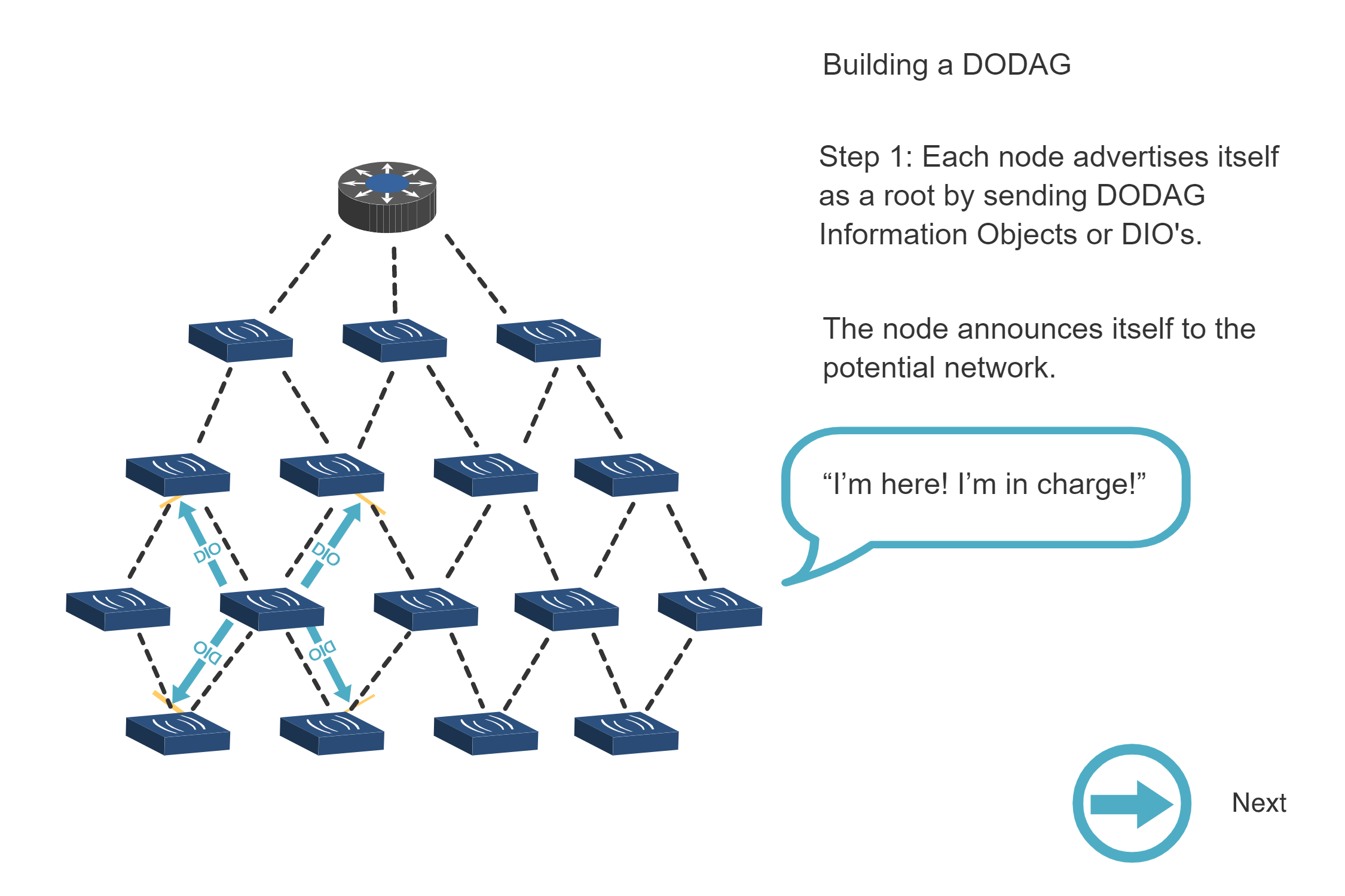
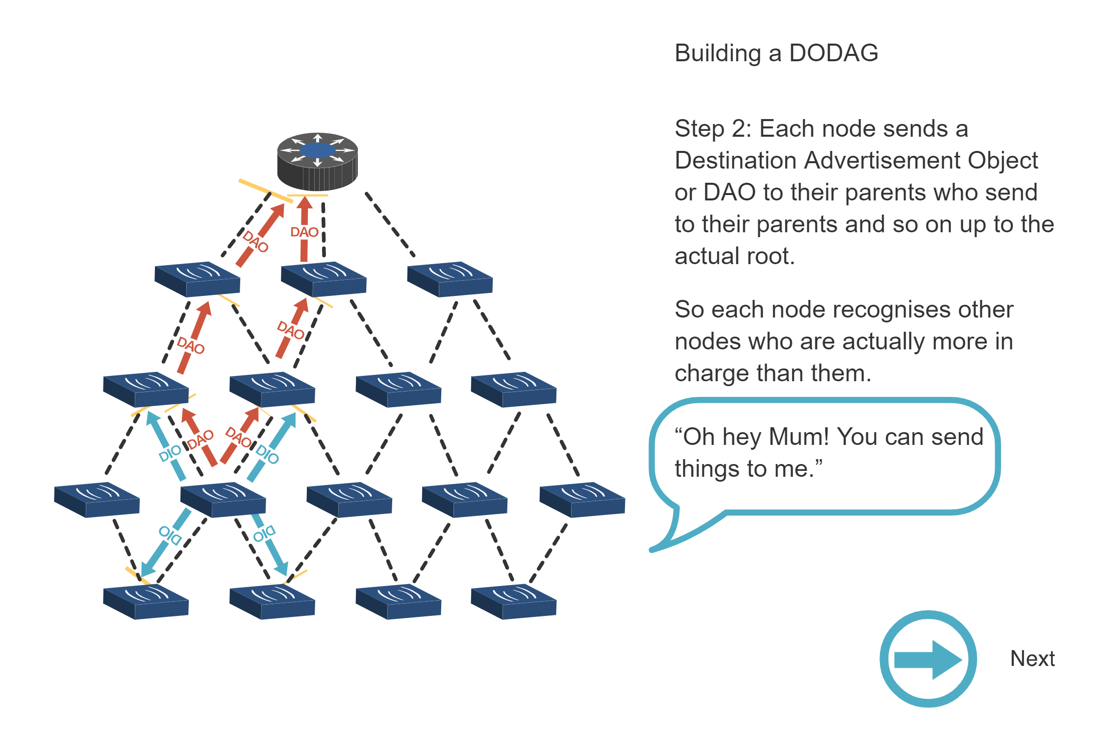
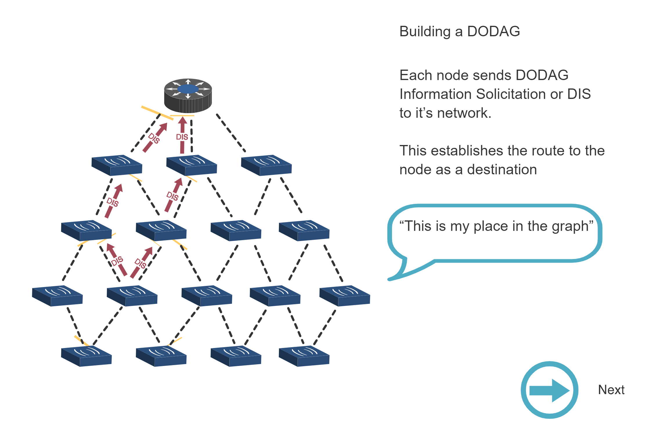
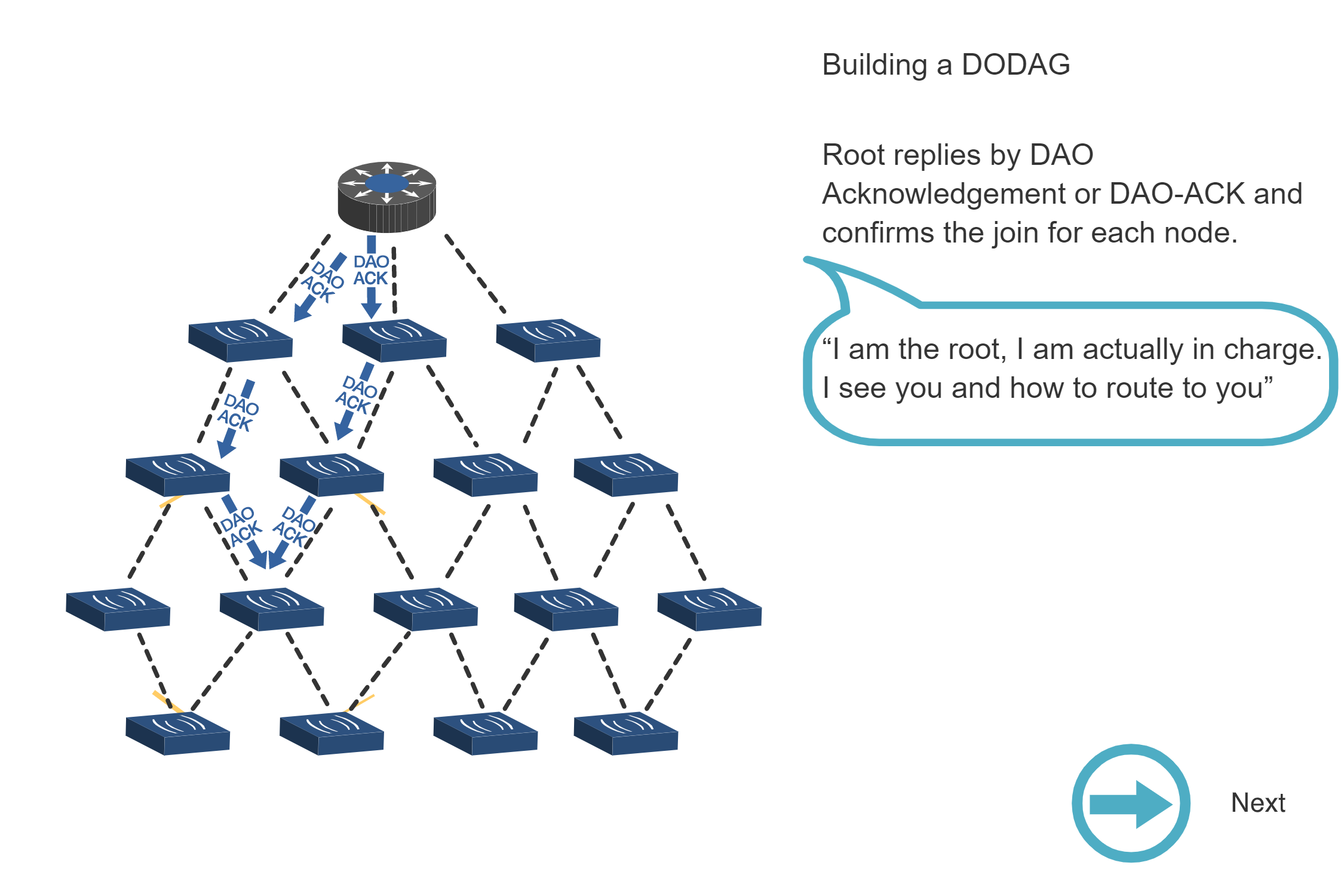
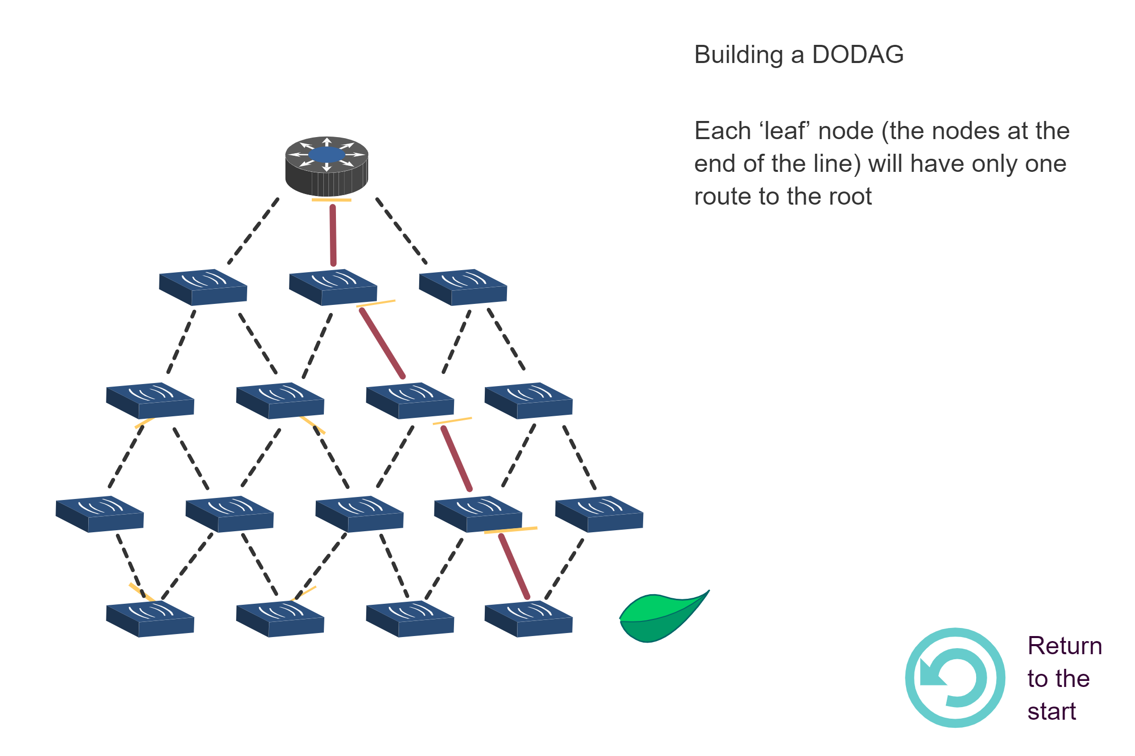
Source: CP IoT System Design Guide, Chapter 4 - Routing

713.4 What’s Next

Continue to RPL Labs and Quiz to apply your understanding through hands-on network design exercises and test your knowledge with comprehensive quiz questions.