%% fig-alt: "Data flow diagram showing tracking pipeline stages: Raw sensor readings from PIR and ultrasonic sensors flow to Detection stage producing binary target present signal. Detection output flows to Cooperation stage where multiple sensor readings are aggregated into fused observations. Fused data flows to Position Computation producing x,y coordinates with uncertainty. Position feeds Prediction stage using Kalman filter to output predicted x,y at time t+delta. Prediction feeds Energy Management which outputs list of sensors to wake. If tracking lost, Recovery stage uses last known position to output expanded search radius."
%%{init: {'theme': 'base', 'themeVariables': { 'primaryColor': '#2C3E50', 'primaryTextColor': '#fff', 'primaryBorderColor': '#16A085', 'lineColor': '#16A085', 'secondaryColor': '#E67E22', 'tertiaryColor': '#7F8C8D'}}}%%
flowchart LR
    subgraph Input["Sensor Inputs"]
        Raw["PIR: motion<br/>Ultrasonic: distance<br/>RSSI: signal strength"]
    end

    subgraph Detection["1. Detection"]
        D["Multi-sensor<br/>Fusion"]
        D_out["Output:<br/>Target Present?<br/>Confidence: 0-1"]
    end

    subgraph Cooperation["2. Cooperation"]
        C["Cluster<br/>Aggregation"]
        C_out["Output:<br/>Fused observations<br/>N sensor reports"]
    end

    subgraph Position["3. Position"]
        P["Trilateration<br/>Least-squares"]
        P_out["Output:<br/>(x, y) ± σ meters"]
    end

    subgraph Prediction["4. Prediction"]
        Pr["Kalman<br/>Filter"]
        Pr_out["Output:<br/>(x', y') at t+Δt<br/>Velocity (vx, vy)"]
    end

    subgraph Energy["5. Energy"]
        E["Selective<br/>Wake-up"]
        E_out["Output:<br/>Sensor IDs to wake<br/>Sleep commands"]
    end

    subgraph Recovery["6. Recovery"]
        R["Expanding<br/>Ring Search"]
        R_out["Output:<br/>Search radius<br/>Wake sequence"]
    end

    Raw --> D --> D_out
    D_out --> C --> C_out
    C_out --> P --> P_out
    P_out --> Pr --> Pr_out
    Pr_out --> E --> E_out
    P_out -.->|"Lost?"| R --> R_out

    style Input fill:#7F8C8D,stroke:#2C3E50,color:#fff
    style Detection fill:#16A085,stroke:#2C3E50,color:#fff
    style Cooperation fill:#16A085,stroke:#2C3E50,color:#fff
    style Position fill:#E67E22,stroke:#2C3E50,color:#fff
    style Prediction fill:#E67E22,stroke:#2C3E50,color:#fff
    style Energy fill:#2C3E50,stroke:#16A085,color:#fff
    style Recovery fill:#2C3E50,stroke:#16A085,color:#fff
395 WSN Tracking: Algorithm Components
395.1 Learning Objectives
By the end of this chapter, you will be able to:
- Implement Target Detection: Design multi-sensor fusion systems to reliably detect targets while minimizing false positives
- Coordinate Node Cooperation: Develop cluster formation and data aggregation strategies for collaborative tracking
- Compute Target Position: Apply trilateration algorithms using distance measurements from multiple sensors
- Estimate Future Positions: Implement Kalman filtering for trajectory prediction and proactive sensor activation
- Compare Localization Techniques: Select appropriate positioning methods based on accuracy and cost requirements
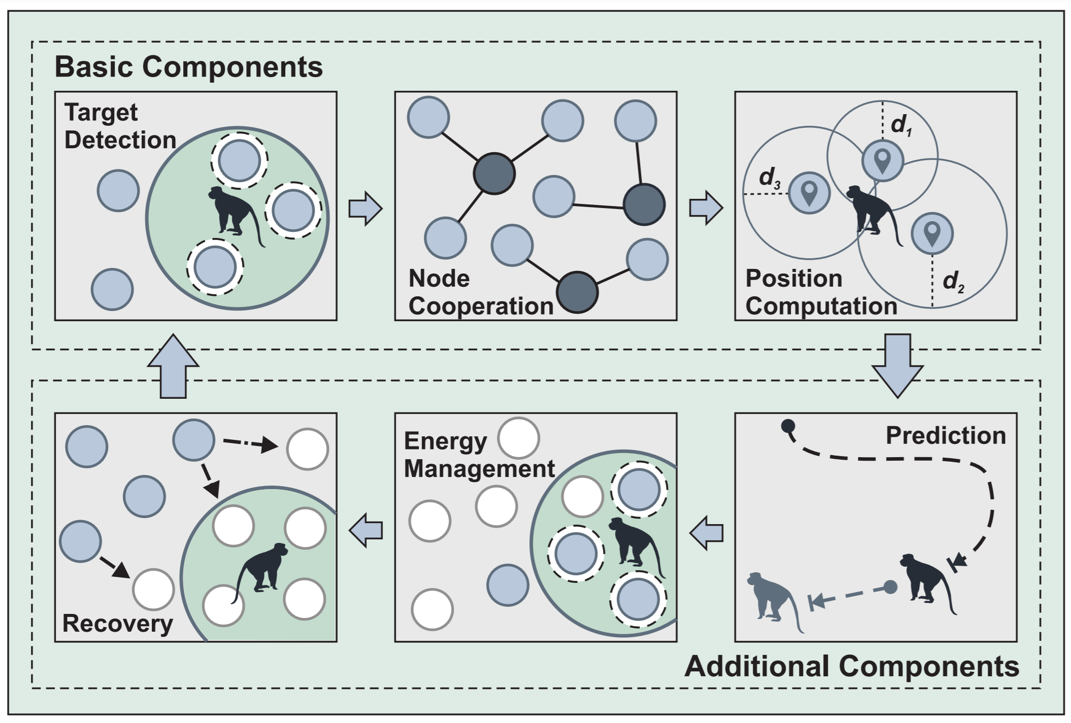
Core concept: WSN tracking algorithms have six key components - detection, cooperation, position computation, prediction, energy management, and recovery. Why it matters: Each component addresses a specific challenge; missing any one can cause tracking failure or excessive energy consumption. Key takeaway: Prediction is the central component - it enables proactive sensor wake-up (energy savings) and guides recovery when tracking fails.
395.2 Prerequisites
Before diving into this chapter, you should be familiar with:
- WSN Tracking: Problem Formulations: Understanding of push, poll, and guided tracking approaches
- WSN Tracking: Fundamentals: Overview of tracking concepts and challenges
- Wireless Sensor Networks: WSN architecture and communication basics
395.3 Components of Target Tracking Algorithms

Effective tracking systems integrate six key components:
This variant shows the data transformation at each stage, making clear what inputs and outputs flow between components.
Data Pipeline Insight: Each stage transforms data—from raw sensor readings to actionable commands. The prediction stage is central because it enables both proactive energy management AND guides recovery when tracking fails.
395.3.1 Target Detection
Challenge: Reliably detect target while minimizing false positives and energy consumption.
Techniques: - Threshold-based detection: Sensor reading > threshold → target present - Multi-sensor fusion: Combine PIR + ultrasonic + temperature for reliability - Adaptive thresholds: Adjust based on environmental conditions
Example: Agricultural Intruder Detection
// Multi-sensor fusion for reliable animal detection
class IntruderDetector {
private:
    int pir_pin, ultrasonic_trig_pin, ultrasonic_echo_pin;
    float detection_threshold_distance = 5.0;  // meters

public:
    IntruderDetector(int pir, int trig, int echo)
        : pir_pin(pir), ultrasonic_trig_pin(trig), ultrasonic_echo_pin(echo) {}

    bool detectTarget() {
        // 1. PIR sensor: motion detection
        bool motion_detected = digitalRead(pir_pin) == HIGH;

        if (!motion_detected) {
            return false;  // No motion, no target
        }

        // 2. Ultrasonic: distance measurement
        float distance = measureDistance();

        if (distance > detection_threshold_distance) {
            return false;  // Too far, likely false positive
        }

        // 3. Multi-sensor fusion: both agree
        Serial.printf("TARGET DETECTED: Motion=YES, Distance=%.2fm\n", distance);
        return true;
    }

    float measureDistance() {
        // Trigger ultrasonic pulse
        digitalWrite(ultrasonic_trig_pin, LOW);
        delayMicroseconds(2);
        digitalWrite(ultrasonic_trig_pin, HIGH);
        delayMicroseconds(10);
        digitalWrite(ultrasonic_trig_pin, LOW);

        // Measure echo duration
        long duration = pulseIn(ultrasonic_echo_pin, HIGH);

        // Calculate distance (speed of sound = 343 m/s)
        float distance = (duration * 0.0343) / 2.0;

        return distance;
    }
};
395.3.2 Node Cooperation
Purpose: Multiple sensors collaborate to reduce communication cost and improve accuracy.
Mechanisms: - Cluster formation: Nearby sensors form temporary groups - In-network aggregation: Fuse data before transmission - Leader election: Select cluster head dynamically
395.3.3 Position Computation
Goal: Estimate target coordinates from sensor measurements.
Methods:
Trilateration (Distance-Based):
\[ (x - x_1)^2 + (y - y_1)^2 = d_1^2 \] \[ (x - x_2)^2 + (y - y_2)^2 = d_2^2 \] \[ (x - x_3)^2 + (y - y_3)^2 = d_3^2 \]
Solve for \((x, y)\) given sensor positions \((x_i, y_i)\) and measured distances \(d_i\).
The Misconception: GPS-based tracking works everywhere.
Why It’s Wrong: - GPS requires line-of-sight to 4+ satellites - Signals blocked by roofs, walls, urban canyons - Indoor accuracy degrades to 10-50m (vs 3m outdoor) - Cold start takes 30+ seconds (longer without sky view) - Power consumption high even when searching
Real-World Example: - Asset tracking in warehouse: - GPS tracker placed on pallet - Signal acquired at loading dock: Position accurate - Moved inside warehouse: Position frozen at last fix - Result: System shows pallet at dock when it’s in storage
The Correct Understanding: | Environment | GPS | Alternatives | |————-|—–|————–| | Outdoor open | ✓ Excellent | - | | Urban canyon | ⚠ Degraded | Wi-Fi, cellular | | Indoor | ✗ Fails | BLE beacons, UWB, Wi-Fi | | Underground | ✗ Fails | UWB, IMU dead reckoning |
Use indoor positioning systems (BLE, UWB, Wi-Fi) for indoor tracking. GPS is outdoor only.
395.3.4 Localization Techniques: A Progressive Journey
Different localization techniques offer different accuracy-complexity tradeoffs:
This variant shows localization options as a cost-benefit decision matrix, helping engineers select the right technique for their budget and accuracy requirements.
%% fig-alt: "XY plot showing localization techniques positioned by hardware cost on X-axis and position accuracy on Y-axis. Cell ID is lowest cost and lowest accuracy at around 100m. RSSI is low cost with 5-10m accuracy. Wi-Fi fingerprinting is medium cost with 2-5m accuracy. ToA/TDoA is medium-high cost with 1-3m accuracy. UWB is high cost with 10-30cm accuracy. Sensor fusion combining IMU with UWB achieves highest accuracy under 10cm at highest cost. Dotted lines show application requirements: warehouse needs 1m, AGV needs 10cm."
%%{init: {'theme': 'base', 'themeVariables': { 'primaryColor': '#2C3E50', 'primaryTextColor': '#fff', 'primaryBorderColor': '#16A085', 'lineColor': '#16A085', 'secondaryColor': '#E67E22', 'tertiaryColor': '#7F8C8D'}}}%%
quadrantChart
    title Localization: Cost vs Accuracy Trade-off
    x-axis Low Cost --> High Cost
    y-axis Low Accuracy --> High Accuracy
    quadrant-1 Premium Solutions
    quadrant-2 Best Value
    quadrant-3 Budget Options
    quadrant-4 Niche Applications

    Cell ID: [0.1, 0.1]
    RSSI: [0.2, 0.3]
    Wi-Fi Fingerprint: [0.35, 0.45]
    ToA TDoA: [0.5, 0.65]
    AoA: [0.65, 0.75]
    UWB: [0.8, 0.85]
    Sensor Fusion: [0.95, 0.95]
Selection Guidance: - Warehouse asset tracking (1m accuracy needed): Wi-Fi fingerprinting or ToA offers best value - AGV navigation (10cm accuracy needed): UWB or sensor fusion required despite higher cost - Smart city (10m acceptable): RSSI-based methods minimize infrastructure cost
| Technique | Accuracy | Hardware Cost | Power | Best For |
|---|---|---|---|---|
| Cell ID | ~100m | None | Lowest | Coarse outdoor |
| RSSI | 5-10m | Standard radios | Low | Indoor zones |
| ToA/TDoA | 1-3m | Precise clocks | Medium | Asset tracking |
| AoA | 0.5-1m | Antenna arrays | High | Precision indoor |
| Fusion | 0.1-0.5m | Multiple sensors | Highest | Robotics, AGV |
Each 10× improvement in accuracy typically requires 10× more hardware cost or power. Choose the minimum accuracy that meets your application requirements.
395.3.5 Future Position Estimation
Purpose: Predict where target will be, enabling proactive sensor activation and tracker guidance.
Kalman Filter Example:
Output:
Predicted: (2.00, 1.00)
Updated:   Position=(2.05, 0.95), Velocity=(2.00, 1.00)

Predicted: (4.05, 1.95)
Updated:   Position=(4.13, 2.03), Velocity=(2.01, 1.02)

Predicted: (6.14, 3.05)
Updated:   Position=(6.02, 2.97), Velocity=(1.97, 0.99)

Predicted: (7.99, 3.96)
Updated:   Position=(8.05, 4.10), Velocity=(2.01, 1.07)
Key Benefit: Kalman filter smooths noisy measurements and provides velocity estimates for prediction.
395.3.6 Energy Management
Strategy: Activate only sensors near predicted target path, letting others sleep.
Prediction-Based Wake-Up:
Energy Savings Calculation:
If target moves through 10% of network area, prediction-based wake-up activates only ~10-15% of nodes, achieving 85-90% energy savings vs. keeping all nodes active.
395.3.7 Target Recovery
Challenge: If prediction fails and target “disappears,” how do we find it again?
Recovery Strategies:
- Expanding ring search: Activate nodes in increasing radius from last known position
- Probabilistic search: Weight search based on target’s historical movement patterns
- Network-wide query: Last resort - wake all nodes briefly
def recover_lost_target(sensors, last_known_position, search_radius_step=10, max_radius=50):
    """Expanding ring search for lost target"""
    print(f"Target lost! Last known: {last_known_position}")
    print("Initiating recovery search...\n")

    for radius in range(search_radius_step, max_radius + 1, search_radius_step):
        print(f"Search radius: {radius}m")

        # Activate sensors in ring
        ring_sensors = [s for s in sensors
                       if radius - search_radius_step <= calculate_distance(s.position, last_known_position) < radius]

        print(f"  Activating {len(ring_sensors)} sensors in ring")

        # Search for target
        for sensor in ring_sensors:
            if sensor.detect_target():
                print(f"✓ TARGET RECOVERED by sensor {sensor.id} at {sensor.position}")
                return sensor.position

    print("✗ Target not found within maximum search radius")
    return None
This completes the six components. Combining them creates robust, energy-efficient tracking systems.
The Misconception: Deploying more sensors always improves tracking accuracy and reliability.
The Reality: Diminishing returns and increased complexity.
Real-World Example - Wildlife Tracking in Yellowstone National Park:
- Initial Deployment (2018): 500 sensors, 20m spacing, tracking elk herds
- Accuracy: 2.5m average position error
- Energy consumption: Network lifetime 6 months
- Data overhead: 15,000 messages/hour during peak movement
- Dense Deployment (2019): 1,500 sensors (3× increase), 10m spacing
- Accuracy: 1.8m average position error (only 28% improvement)
- Energy consumption: Network lifetime 2 months (67% reduction)
- Data overhead: 85,000 messages/hour (5.7× increase)
- Communication collisions: Increased by 340%
- Cost: 3× sensor hardware + 4× deployment labor
Why This Happens:
Localization accuracy saturates: Once you have 3-4 sensors detecting target, additional sensors provide marginal accuracy gains due to geometric dilution of precision (GDOP)
Communication overhead explodes: More sensors = more messages → more collisions → more retransmissions → faster battery drain
Cluster formation overhead: With dense deployments, cluster head election and data aggregation take longer, increasing latency
Optimal Approach - Adaptive Density:
Instead of uniform high density, Yellowstone researchers deployed: - High density (10m spacing) in critical areas: river crossings, migration bottlenecks - Low density (30m spacing) in open terrain: meadows, forests - Prediction-based activation: Only wake nearby sensors based on trajectory prediction
Results (2020 optimized deployment): - Sensors: 650 total (30% fewer than original) - Accuracy: 2.2m average (comparable to dense deployment) - Network lifetime: 14 months (2.3× original) - Cost savings: $125,000 vs $280,000 for dense approach
Key Lesson: Tracking performance depends on smart algorithms (prediction, selective activation, data fusion) more than raw sensor count. Focus on strategic placement and energy-efficient coordination rather than brute-force density.
395.4 Summary
This chapter covered the six essential components of WSN target tracking algorithms:
Target Detection: Multi-sensor fusion combining PIR motion, ultrasonic ranging, and temperature sensing reduces false positives and improves detection reliability.
Node Cooperation: Cluster formation and in-network data aggregation enable sensors to collaborate, reducing communication overhead while improving position accuracy.
Position Computation: Trilateration using distance measurements from 3+ sensors enables precise position estimation, with least-squares optimization for noisy measurements.
Future Position Estimation: Kalman filtering provides smooth trajectory prediction by combining motion models with noisy measurements, enabling proactive sensor activation.
Energy Management: Prediction-based selective wake-up activates only sensors along the expected target path, achieving 85-90% energy savings.
Target Recovery: Expanding ring search and probabilistic methods relocate targets when predictions fail, ensuring robust tracking despite unpredictable target behavior.
395.5 What’s Next
Continue to the next chapter to see a Worked Example of Predictive Sensor Activation that demonstrates how these components work together in a real-world parking lot tracking scenario, with detailed calculations showing 95% energy savings.


