%% fig-alt: "Routing protocol decision tree starting with network type (static or mobile), then for static networks checking node density, if dense checking hierarchy needs to select LEACH for clustered topology or PEGASIS for linear topology, if no hierarchy use Directed Diffusion, if sparse use SPIN flat routing, if mobile use AODV reactive routing"
%%{init: {'theme': 'base', 'themeVariables': { 'primaryColor': '#2C3E50', 'primaryTextColor': '#fff', 'primaryBorderColor': '#16A085', 'lineColor': '#16A085', 'secondaryColor': '#E67E22', 'tertiaryColor': '#7F8C8D'}}}%%
graph TB
    Start{Network<br/>Type?}

    Start --> |Static| Static{Nodes<br/>Dense?}
    Start --> |Mobile| Mobile["Use AODV<br/>Reactive routing"]

    Static --> |Yes Dense| Dense{Need<br/>Hierarchy?}
    Static --> |No Sparse| Sparse["Use SPIN<br/>Flat routing"]

    Dense --> |Yes| Cluster{Topology?}
    Dense --> |No| Flat["Use Directed<br/>Diffusion"]

    Cluster --> |Clustered| LEACH["Use LEACH<br/>Cluster-based"]
    Cluster --> |Linear| PEGASIS["Use PEGASIS<br/>Chain-based"]

    style Start fill:#2C3E50,stroke:#16A085,color:#fff
    style Static fill:#2C3E50,stroke:#16A085,color:#fff
    style Dense fill:#2C3E50,stroke:#16A085,color:#fff
    style Cluster fill:#2C3E50,stroke:#16A085,color:#fff
    style LEACH fill:#16A085,stroke:#2C3E50,color:#fff
    style PEGASIS fill:#16A085,stroke:#2C3E50,color:#fff
    style Flat fill:#E67E22,stroke:#2C3E50,color:#fff
    style Sparse fill:#E67E22,stroke:#2C3E50,color:#fff
    style Mobile fill:#E67E22,stroke:#2C3E50,color:#fff
383 WSN Implementation: Routing and Monitoring
383.1 Learning Objectives
By the end of this chapter, you will be able to:
- Select Routing Protocols: Choose appropriate routing algorithms (LEACH, PEGASIS, SPIN, Directed Diffusion, AODV) based on network characteristics
- Apply Decision Frameworks: Use structured decision trees to match protocols to deployment requirements
- Design Monitoring Systems: Implement health dashboards tracking battery levels, packet delivery, and latency
- Configure Failure Detection: Set up heartbeat monitoring and automatic recovery mechanisms for network resilience
383.2 Prerequisites
Before diving into routing and monitoring, you should be familiar with:
- WSN Implementation: Architecture and Topology: Multi-tier system design and cluster topology concepts
- WSN Implementation: Deployment and Energy: Sensor placement and energy management strategies
383.3 Routing Protocol Selection
383.3.1 Protocol Comparison
Different WSN routing protocols optimize for different deployment scenarios:
| Protocol | Type | Energy Efficiency | Scalability | Best For |
|---|---|---|---|---|
| LEACH | Hierarchical | High | Medium | Static networks |
| PEGASIS | Chain | Very High | Low | Linear deployments |
| SPIN | Flat | Medium | High | Event-driven |
| Directed Diffusion | Data-centric | High | High | Query-response |
| AODV | Reactive | Low | High | Mobile networks |
Protocol Details:
TipLEACH (Low-Energy Adaptive Clustering Hierarchy)
How it works: Nodes self-organize into clusters with rotating cluster heads that aggregate data before transmitting to the base station.
Strengths: - Distributes energy load through cluster head rotation - Data aggregation reduces transmission count - Simple distributed algorithm
Weaknesses: - Assumes uniform node distribution - Single-hop from nodes to cluster head - Random cluster head selection can be suboptimal
Best for: Dense, static deployments with uniform distribution (environmental monitoring, smart agriculture)
TipPEGASIS (Power-Efficient Gathering in Sensor Information Systems)
How it works: Nodes form a chain where each node transmits only to its nearest neighbor. One node per round becomes the leader and transmits to the base station.
Strengths: - Minimizes transmission distance - Very energy-efficient for linear deployments - Simple neighbor-to-neighbor communication
Weaknesses: - Chain construction overhead - Single point of failure if chain breaks - High latency for large chains
Best for: Linear deployments (pipeline monitoring, highway sensors, perimeter security)
TipSPIN (Sensor Protocols for Information via Negotiation)
How it works: Nodes use negotiation to eliminate redundant data transmission. ADV (advertisement), REQ (request), and DATA messages coordinate transfers.
Strengths: - Avoids duplicate data transmission - Works well for event-driven data - No topology constraints
Weaknesses: - Higher control message overhead - No guarantee of data delivery - Doesn’t consider remaining energy
Best for: Event-driven applications where data redundancy is common (intrusion detection, fire monitoring)
TipDirected Diffusion
How it works: Base station floods “interests” (queries) into the network. Data matching interests flows back along reinforced gradient paths.
Strengths: - Data-centric naming (query what you want) - In-network aggregation - Path repair through gradient refresh
Weaknesses: - Interest flooding overhead - Not suitable for continuous monitoring - Complex state maintenance
Best for: Query-response applications (find specific events, location-based queries)
TipAODV (Ad-hoc On-Demand Distance Vector)
How it works: Routes discovered only when needed through RREQ/RREP flooding. Routes maintained until broken or expired.
Strengths: - Works with mobile nodes - No periodic routing updates - Adapts to topology changes
Weaknesses: - Route discovery delay - High overhead in high-mobility scenarios - Not optimized for energy
Best for: Mobile sensor networks, vehicular networks, scenarios with frequent topology changes
383.3.2 Routing Decision Matrix
Use this decision tree to select the appropriate protocol:
Quick Selection Guide:
| Deployment Scenario | Recommended Protocol | Reasoning |
|---|---|---|
| Environmental monitoring (100+ static sensors) | LEACH | Clustering handles scale, rotation balances energy |
| Pipeline monitoring (linear sensors) | PEGASIS | Chain topology matches physical layout |
| Wildlife tracking (mobile sensors) | AODV | Handles mobility and topology changes |
| Intrusion detection (event-based) | SPIN | Negotiation prevents redundant alerts |
| Target tracking queries | Directed Diffusion | Query-response matches application pattern |
383.4 Network Monitoring Implementation
383.4.1 Health Metrics Dashboard
A WSN monitoring system tracks key performance indicators:
%% fig-alt: "WSN monitoring system showing three nodes reporting battery levels (85%, 42%, 15%) and packet delivery ratios (98%, 92%, 76%) to monitoring dashboard with metric collector, analytics engine checking thresholds for battery under 20%, PDR under 80%, and latency over 5 seconds, triggering alert system that leads to actions like replacing low battery nodes, diagnosing poor links, adding relay nodes, and adjusting duty cycle"
%%{init: {'theme': 'base', 'themeVariables': { 'primaryColor': '#2C3E50', 'primaryTextColor': '#fff', 'primaryBorderColor': '#16A085', 'lineColor': '#16A085', 'secondaryColor': '#E67E22', 'tertiaryColor': '#7F8C8D'}}}%%
graph TB
    subgraph Nodes["WSN Nodes (send metrics)"]
        N1["Node 1<br/>Battery: 85%<br/>PDR: 98%"]
        N2["Node 2<br/>Battery: 42%<br/>PDR: 92%"]
        N3["Node 3<br/>Battery: 15%<br/>PDR: 76%"]
    end

    subgraph Monitor["Monitoring Dashboard"]
        Collect["Metric Collector"]
        Analyze["Analytics Engine"]
        Alert["Alert System"]
    end

    N1 & N2 & N3 --> |Heartbeat| Collect
    Collect --> Analyze
    Analyze --> |Battery < 20%| Alert
    Analyze --> |PDR < 80%| Alert
    Analyze --> |Latency > 5s| Alert

    Alert --> Action["Actions:<br/>✓ Replace low battery nodes<br/>✓ Diagnose poor links<br/>✓ Add relay nodes<br/>✓ Adjust duty cycle"]

    style N1 fill:#16A085,stroke:#2C3E50,color:#fff
    style N2 fill:#E67E22,stroke:#2C3E50,color:#fff
    style N3 fill:#E67E22,stroke:#2C3E50,color:#fff
    style Collect fill:#2C3E50,stroke:#16A085,color:#fff
    style Analyze fill:#2C3E50,stroke:#16A085,color:#fff
    style Alert fill:#E67E22,stroke:#2C3E50,color:#fff
    style Action fill:#7F8C8D,stroke:#2C3E50,color:#fff
383.4.2 Key Performance Indicators
| Metric | Target | Critical Threshold | Action |
|---|---|---|---|
| Battery Level | >30% | <10% | Replace node |
| Packet Delivery | >95% | <80% | Diagnose link |
| End-to-End Latency | <1 sec | >5 sec | Add relay |
| Coverage | >98% | <90% | Deploy more nodes |
| Network Lifetime | Maximize | - | Optimize duty cycle |
Metric Collection Strategy:
HEARTBEAT MESSAGE STRUCTURE
═══════════════════════════════════════

Message Type: HEARTBEAT (0x01)
Frequency: Every 60 seconds
Size: 16 bytes

Fields:
├── Node ID (2 bytes)
├── Sequence Number (2 bytes)
├── Battery Voltage (2 bytes, mV)
├── Temperature (2 bytes, 0.1°C)
├── Packets Sent (2 bytes, since last HB)
├── Packets Received (2 bytes, since last HB)
├── RSSI to Parent (1 byte, dBm)
├── Hop Count to Gateway (1 byte)
└── Uptime (2 bytes, minutes)

Overhead: 16 bytes × 1440/day = 23 KB/day per node
383.4.3 Failure Detection and Recovery
Common detection methods:
- Heartbeat timeouts - a node stops sending periodic beacons.
- Path quality degradation - sharply increased loss or latency.
- Coverage gaps - regions where no recent readings are received.
- Battery alarms - nodes reporting critically low battery.
Detection Algorithm:
FAILURE DETECTION ALGORITHM
═══════════════════════════════════════

For each node n:
  last_heartbeat[n] = timestamp of last received heartbeat
  missed_count[n] = consecutive missed heartbeats

Every heartbeat_interval:
  For each node n:
    If time_now - last_heartbeat[n] > heartbeat_interval:
      missed_count[n] += 1
    Else:
      missed_count[n] = 0

    If missed_count[n] >= 3:
      mark_node_failed(n)
      notify_operator(n, "Node unresponsive")
      initiate_route_repair(n)
Automatic Recovery Responses:
| Failure type | Automatic response | Manual escalation |
|---|---|---|
| Single node | Route around the failed node; mark for maintenance | After 24 hours |
| Cluster head | Re-elect a new cluster head in that region | If re-election fails |
| Gateway | Switch to a backup gateway if available | Immediate if no backup |
| Regional outage | Raise alert for investigation | Immediate |
Recovery Workflow:
%% fig-alt: "Failure recovery workflow showing detection of node failure leading to route repair attempt, if successful marking node for maintenance, if failed checking for backup path, if backup exists using alternate route, if no backup alerting operator for manual intervention"
%%{init: {'theme': 'base', 'themeVariables': { 'primaryColor': '#2C3E50', 'primaryTextColor': '#fff', 'primaryBorderColor': '#16A085', 'lineColor': '#16A085', 'secondaryColor': '#E67E22', 'tertiaryColor': '#7F8C8D'}}}%%
flowchart TB
    Detect["Detect<br/>Node Failure"]
    Route["Attempt<br/>Route Repair"]
    Success{Repair<br/>Success?}
    Backup{Backup<br/>Path?}
    Maintain["Mark for<br/>Maintenance"]
    Alternate["Use<br/>Alternate Route"]
    Escalate["Alert<br/>Operator"]

    Detect --> Route
    Route --> Success
    Success -->|Yes| Maintain
    Success -->|No| Backup
    Backup -->|Yes| Alternate
    Backup -->|No| Escalate
    Alternate --> Maintain

    style Detect fill:#E67E22,stroke:#2C3E50,color:#fff
    style Route fill:#2C3E50,stroke:#16A085,color:#fff
    style Maintain fill:#16A085,stroke:#2C3E50,color:#fff
    style Alternate fill:#16A085,stroke:#2C3E50,color:#fff
    style Escalate fill:#E67E22,stroke:#2C3E50,color:#fff
383.5 Knowledge Check
NoteQuestion 1: Protocol Selection
A factory needs to deploy 200 sensors across a 10,000 m² floor. Mains power is available at multiple locations. Communication range per node is 30m. Which deployment strategy is most appropriate?
With mains power available, adding gateways is usually simpler and more reliable than making battery sensors relay traffic.
| Strategy | Battery Life | Complexity | Reliability |
|---|---|---|---|
| Full Mesh | 14 hours (routing overhead) | Very High | Appears high, fails fast |
| Star (multiple GW) | 5+ years (no relay burden) | Low | High (gateway redundancy) |
| Single GW | 2+ years | Very Low | Low (single point of failure) |
| Chain | 6 months (relay burden) | Medium | Very Low |
Rule of thumb: “Can I add more gateways instead of mesh routing?” When the answer is yes (mains power available), star topology is almost always superior.
NoteQuestion 2: Routing Protocol Match
A linear pipeline monitoring system with 50 sensors spaced 100m apart needs maximum energy efficiency. Which protocol is most appropriate?
PEGASIS forms a chain where each node transmits only to its nearest neighbor, minimizing transmission distance. This matches the linear physical layout of pipeline monitoring perfectly, achieving very high energy efficiency.
NoteQuestion 3: Failure Detection
A node sends heartbeats every 60 seconds. After how many consecutive missed heartbeats should the system mark the node as failed?
3 consecutive missed heartbeats (3 minutes) provides a balance between quick detection and avoiding false positives from temporary interference or packet loss. 1-2 misses could be normal packet loss, while 10 misses (10 minutes) is too slow for timely response.
383.6 Academic Resources: WSN in Smart Grid Applications
The following academic resources from NPTEL (IIT Kharagpur) illustrate real-world WSN implementations in smart grid infrastructure, demonstrating how wireless sensor networks enable intelligent power distribution and energy management.
NoteAcademic Resource: Smart Grid Network Architecture (NPTEL IoT Course)
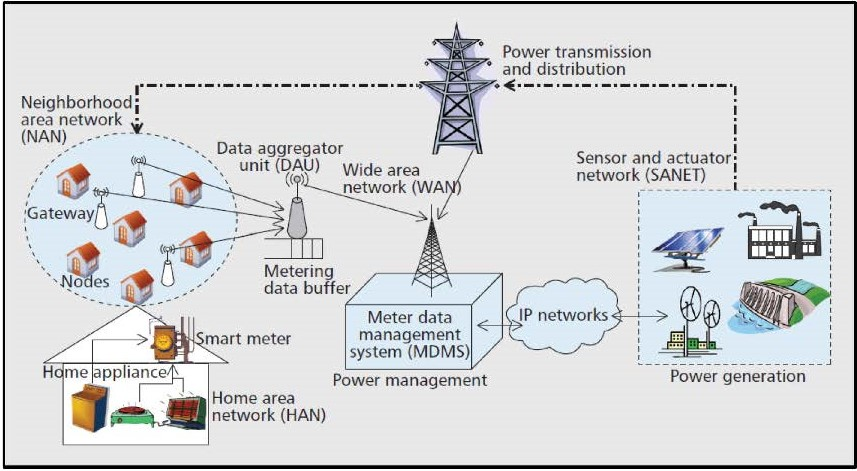
Source: NPTEL Internet of Things Course, IIT Kharagpur
This diagram illustrates the hierarchical WSN architecture used in smart grids:
- HAN (Home Area Network): Connects smart meters and home appliances
- NAN (Neighborhood Area Network): Aggregates data from multiple homes via gateway nodes
- WAN (Wide Area Network): Backbone connecting neighborhoods to utility control centers
- SANET: Sensor/actuator networks monitoring power generation assets
NoteAcademic Resource: Smart Grid Conceptual Model (NPTEL IoT Course)
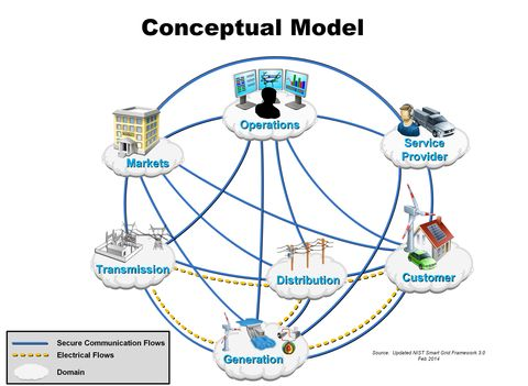
Source: NPTEL Internet of Things Course, IIT Kharagpur
This conceptual model shows how WSN enables communication across all smart grid domains:
- Secure Communication Flows (blue lines): Data exchange between domains
- Electrical Flows (orange lines): Power distribution paths
- Domain Integration: Operations, Markets, Service Provider, Customer, Distribution, Generation, and Transmission all connected through sensor networks
NoteAcademic Resource: WSN Mesh Topology for Smart Grid (NPTEL IoT Course)

Source: NPTEL Internet of Things Course, IIT Kharagpur
This illustration shows practical WSN mesh deployment:
- Mesh Connectivity: Each node connects to multiple neighbors for redundancy
- Central Aggregation: Substation serves as gateway to utility network
- Coverage Pattern: Distributed sensor placement across service area
NoteAcademic Resource: Micro-grid Architecture with Cloud Integration (NPTEL IoT Course)
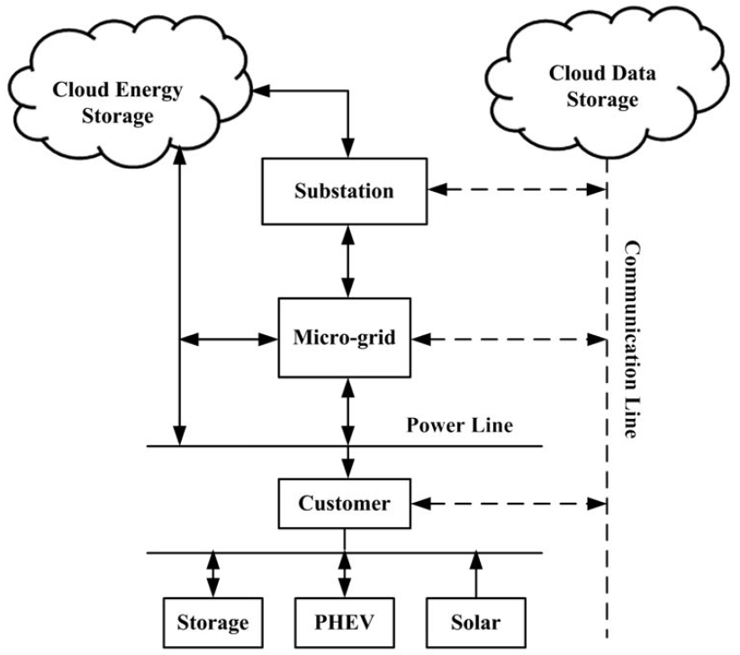
Source: NPTEL Internet of Things Course, IIT Kharagpur
This diagram demonstrates WSN-enabled micro-grid management:
- Power Lines (solid arrows): Bidirectional energy flow
- Communication Lines (dashed arrows): WSN sensor data and control signals
- Customer Integration: Local storage, electric vehicles, and solar generation monitored via sensors
- Cloud Integration: Both energy and data storage in cloud infrastructure
383.7 Summary
This chapter covered WSN routing protocol selection and network monitoring:
- Protocol Selection: LEACH for static clustered networks, PEGASIS for linear deployments, SPIN for event-driven, Directed Diffusion for queries, AODV for mobile networks
- Decision Framework: Use structured decision trees based on mobility, density, topology, and application pattern to select appropriate protocols
- Health Monitoring: Track battery levels (>30%), packet delivery (>95%), latency (<1s), and coverage (>98%) with automated alerts
- Failure Detection: Heartbeat timeouts with 3-miss threshold balance quick detection against false positives
- Automatic Recovery: Route repair, cluster head re-election, and backup gateway switching minimize manual intervention
383.8 What’s Next
Continue to WSN Overview: Review for a comprehensive summary of WSN concepts, advanced topics, and review exercises covering all implementation aspects.
NoteRelated Chapters
Implementation Series: - WSN Implementation: Architecture and Topology - System design fundamentals - WSN Implementation: Deployment and Energy - Coverage and power management
Fundamentals: - WSN Overview: Fundamentals - Core sensor network concepts - Wireless Sensor Networks - WSN architecture principles
Protocols: - RPL Routing - IoT routing protocol for WSNs - 6LoWPAN - IPv6 over low-power networks - MQTT - Lightweight messaging for sensors
Reviews: - WSN Overview: Review - Comprehensive WSN summary - Networking Review - Protocol comparison guide
Learning: - Simulations Hub - WSN simulation tools and frameworks - Design Strategies - Network planning approaches
383.9 Visual Reference Gallery
NoteWSN Implementation Visualizations
These AI-generated figures provide alternative visual representations of WSN implementation concepts covered in this chapter.
383.9.1 Sensor Network Architecture

383.9.2 Basic Sensor Node Components

383.9.3 Fog Node Hierarchy
