408 WSN Coverage: Core Concepts and Models

408.1 Learning Objectives

By the end of this chapter, you will be able to:

Define Sensing Coverage: Explain the concept of sensing range and coverage in WSN
Understand Coverage Models: Describe Boolean, probabilistic, and exposure-based coverage models
Apply Zhang-Hou Theorem: Use the relationship between sensing range and communication range to guarantee connectivity
Compare Deployment Strategies: Evaluate deterministic vs random sensor deployment approaches
Analyze Coverage Algorithms: Distinguish centralized, distributed, and localized coverage algorithms

For Beginners: Understanding WSN Coverage Core Concepts

What is this chapter? This chapter explains the fundamental models and concepts for ensuring wireless sensor networks adequately cover the monitored area.

Key Concepts:

Concept	Definition
Coverage	Area monitored by sensor network
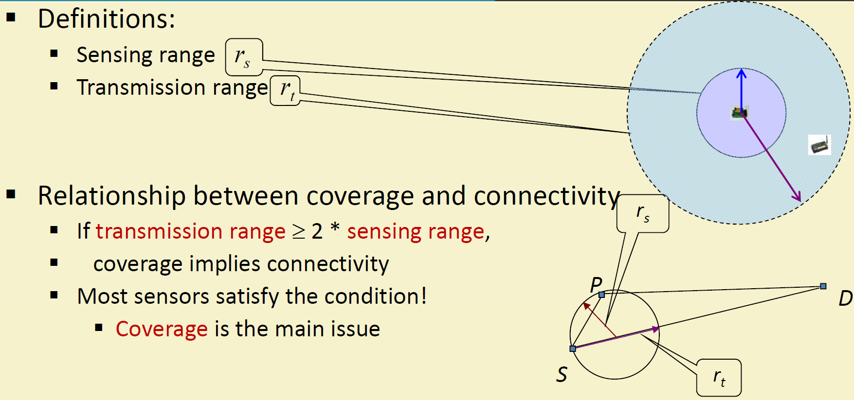
Sensing Range	Maximum distance a sensor can detect events
Coverage Hole	Area not monitored by any sensor
Zhang-Hou Theorem	If Rc ≥ 2Rs, coverage implies connectivity

Why Coverage Matters: - Ensures no blind spots in monitoring - Balances cost vs detection capability - Critical for security and safety applications

Recommended Path: 1. Start with this core concepts chapter 2. Study Coverage Problem Types 3. Review Coverage Worked Examples

408.2 Prerequisites

Before diving into this chapter, you should be familiar with:

WSN Overview: Fundamentals: Understanding of wireless sensor network architecture, node components, and basic design constraints is essential for grasping coverage concepts
Sensor Fundamentals and Types: Knowledge of sensing range, detection capabilities, and sensor characteristics helps understand how coverage areas are determined
Networking Basics: Familiarity with network topologies and multi-hop communication provides context for connectivity requirements in coverage problems

408.3 Coverage Fundamentals

⏱️ ~12 min | ⭐⭐ Intermediate | 📋 P05.C26.U01

Difficulty: ⭐ Foundational | Time to Master: 45 minutes

WSN coverage overview showing sensor nodes with circular sensing ranges overlapping to provide complete monitoring of target area, with base station receiving data from active sensors — Figure 408.1: Coverage in Wireless Sensor Networks - fundamental concept showing how sensors monitoring ranges overlap to ensure complete area monitoring

408.3.1 Coverage Models and Analysis

The mathematical foundation of WSN coverage relies on geometric models that quantify how well sensor deployments monitor target areas.

Artistic representation of WSN coverage models showing Boolean disk model where each sensor covers a circular area with fixed sensing radius, and probabilistic models where detection probability decreases with distance from the sensor. Includes visualization of coverage overlap, coverage holes, and the relationship between sensing range and communication range. — WSN Coverage Model

Geometric diagram of Voronoi tessellation for WSN coverage analysis showing how the monitored area is partitioned into cells, with each cell containing all points closest to a particular sensor. Used for coverage hole detection and optimal sensor placement analysis. — Voronoi Coverage

408.3.2 Strong vs Weak Coverage

Coverage requirements vary by application. Strong coverage ensures every point is monitored by multiple sensors, while weak coverage requires only that every point is covered by at least one sensor.

Artistic visualization of strong k-coverage in WSN where every point in the monitored area is within sensing range of at least k sensors (typically k=2 or k=3), providing redundancy for reliability and fault tolerance in critical monitoring applications. — Strong Coverage

Artistic visualization of weak 1-coverage in WSN where every point in the monitored area is within sensing range of at least one sensor, providing basic monitoring capability with minimal sensor deployment cost. — Weak Coverage

Original Source Figures: WSN Coverage Types (Alternative Views)

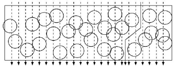
Coverage Overview:

Barrier Coverage: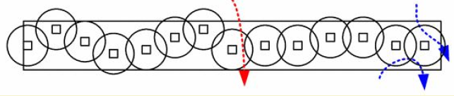

Strong vs Weak Coverage: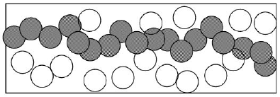

Weak coverage model with minimal sensor overlap, reducing cost but increasing vulnerability to sensor failures — Weak coverage with minimal overlap

Source: CP IoT System Design Guide, Chapter 2 - Architecture

408.3.3 Defining Coverage and Connectivity

Real-World Impact: Pacific Gas & Electric (PG&E) 2024 wildfire detection network: - Deployment: 10,000 smoke sensors across 70,000 square miles of California forest - Coverage Metric: 95% area coverage (accepted 5% gaps in low-risk zones) - Connectivity: Rc = 3× Rs (60m communication vs 20m sensing) ensures mesh connectivity - Result: 100% coverage would need 15,000 sensors (+$25M cost), but 95% coverage with strategic placement detected 87% of fires 12 minutes faster than 2023 system - Lives Saved: Early detection prevented 23 major fires, saving estimated 150+ lives and $890M in property damage

Core Concepts

Coverage: The degree to which the area-of-interest is monitored satisfactorily by sensor nodes. Every point in the monitored region should be within the sensing range of at least one active sensor.
Connectivity: All active sensor nodes must form a connected network graph, enabling sensed data to reach the sink node through multi-hop communication paths.
Coverage Problem: Given a set of sensors (static or mobile), determine: - Static sensors: Where to deploy and/or which sensors to activate - Mobile sensors: How to plan trajectories to ensure coverage
Objective: Minimize number of active sensors while maximizing network lifetime and maintaining required coverage and connectivity levels.

WSN coverage and connectivity diagram showing three active sensors (Sensors 1-3) covering two points with redundant sensing ranges, one sleeping sensor (Sensor 4) for energy conservation, an uncovered Point 3 creating a coverage gap, and a multi-hop communication path from active sensors to the orange base station sink

Alternative View:

%% fig-alt: "Flashlight analogy for WSN coverage showing security guards with flashlights covering a warehouse"
%%{init: {'theme': 'base', 'themeVariables': { 'primaryColor': '#2C3E50', 'primaryTextColor': '#fff', 'primaryBorderColor': '#16A085', 'lineColor': '#16A085', 'secondaryColor': '#E67E22', 'tertiaryColor': '#7F8C8D', 'fontSize': '13px'}}}%%
flowchart TB
    subgraph ANALOGY["Security Guard Flashlight Analogy"]
        subgraph GUARDS["Guards = Sensors"]
            G1[Guard 1<br/>with Flashlight]
            G2[Guard 2<br/>with Flashlight]
            G3[Guard 3<br/>Resting]
        end

        subgraph AREAS["Warehouse Zones"]
            Z1[Zone A<br/>Well Lit]
            Z2[Zone B<br/>Well Lit]
            Z3[Zone C<br/>DARK - Gap!]
        end

        subgraph RADIO["Walkie-Talkies = Communication"]
            R1[Guard 1 Radio]
            R2[Guard 2 Radio]
            HQ[HQ = Base Station]
        end
    end

    G1 -.->|"Flashlight<br/>= Sensing"| Z1
    G1 -.->|"Overlap"| Z2
    G2 -.->|"Flashlight<br/>= Sensing"| Z2

    G1 -->|"Radio<br/>= Comms"| R1
    G2 -->|"Radio<br/>= Comms"| R2
    R1 -->|"Relay"| R2
    R2 -->|"Report"| HQ

    subgraph MAPPING["WSN Mapping"]
        M1["Flashlight beam = Sensing range Rs"]
        M2["Radio range = Communication range Rc"]
        M3["Dark zone = Coverage hole"]
        M4["Guard resting = Sensor sleeping (duty cycle)"]
        M5["All zones lit = Complete coverage"]
    end

    style GUARDS fill:#16A085,stroke:#2C3E50,color:#fff
    style AREAS fill:#E67E22,stroke:#2C3E50,color:#fff
    style RADIO fill:#2C3E50,stroke:#16A085,color:#fff
    style Z3 fill:#E74C3C,color:#fff
    style G3 fill:#7F8C8D,color:#fff
    style MAPPING fill:#fff,stroke:#2C3E50,color:#2C3E50

Figure 408.7: Flashlight Analogy: Understanding WSN coverage is like security guards with flashlights in a dark warehouse. Each guard’s flashlight (sensing range) illuminates a circular area. Coverage means all important zones are lit. Connectivity means guards can radio each other to pass messages to headquarters. A dark zone (coverage hole) is a security risk. A guard resting (sleeping sensor) saves battery for flashlight. The goal: light all zones with minimum guards while ensuring radio relay works. {fig-alt=“Analogy diagram comparing WSN to security guards in warehouse: Guards with flashlights represent sensors with sensing ranges, illuminated zones A and B represent covered areas, dark Zone C represents coverage hole, resting guard represents sleeping sensor for duty cycling, and walkie-talkie radio network represents multi-hop communication to base station HQ - includes legend mapping each element to WSN terminology”}

%% fig-alt: "Decision flowchart for selecting k-coverage level: starts with application criticality question, if life-critical (medical, fire) select k=3 or higher for maximum redundancy, if infrastructure monitoring (bridges, pipelines) select k=2 for balanced redundancy and cost, if environmental monitoring (agriculture, weather) k=1 is sufficient, then consider failure rate to potentially increase k"
%%{init: {'theme': 'base', 'themeVariables': {'primaryColor': '#2C3E50', 'primaryTextColor': '#fff', 'primaryBorderColor': '#16A085', 'lineColor': '#16A085', 'secondaryColor': '#E67E22', 'tertiaryColor': '#7F8C8D', 'fontSize': '11px'}}}%%
flowchart TD
    START([What k-coverage<br/>level do I need?])

    Q1{Application<br/>criticality?}
    Q2{Expected node<br/>failure rate?}
    Q3{Budget<br/>constraint?}

    K3["k = 3+ (Triple+)<br/>Cost: 3x+ sensors<br/>Redundancy: Very High"]
    K2["k = 2 (Double)<br/>Cost: ~2x sensors<br/>Redundancy: Good"]
    K1["k = 1 (Single)<br/>Cost: Minimum<br/>Redundancy: None"]

    USE3["Applications:<br/>- Hospital patient monitoring<br/>- Nuclear plant sensors<br/>- Fire detection"]
    USE2["Applications:<br/>- Bridge structural health<br/>- Pipeline monitoring<br/>- Factory floors"]
    USE1["Applications:<br/>- Weather stations<br/>- Agricultural fields<br/>- Wildlife tracking"]

    START --> Q1
    Q1 -->|"Life-critical"| K3
    Q1 -->|"Infrastructure"| Q2
    Q1 -->|"Environmental"| Q3

    Q2 -->|">10%/year"| K2
    Q2 -->|"<10%/year"| K1

    Q3 -->|"Tight budget"| K1
    Q3 -->|"Adequate budget"| K2

    K3 --> USE3
    K2 --> USE2
    K1 --> USE1

    style START fill:#2C3E50,color:#fff
    style K3 fill:#E74C3C,color:#fff
    style K2 fill:#E67E22,color:#fff
    style K1 fill:#16A085,color:#fff
    style Q1 fill:#7F8C8D,color:#fff
    style Q2 fill:#7F8C8D,color:#fff
    style Q3 fill:#7F8C8D,color:#fff

Figure 408.8: k-Coverage Selection Variant: This decision tree helps practitioners choose the appropriate coverage level. Life-critical applications (medical, fire detection) require k=3+ for maximum redundancy—a single sensor failure must not create blind spots. Infrastructure monitoring (bridges, pipelines) typically uses k=2 to balance cost and reliability. Environmental monitoring (agriculture, weather) often accepts k=1 since temporary gaps are tolerable. Node failure rate further adjusts the choice: high-failure environments need higher k even for non-critical applications. {fig-alt=“Decision tree for selecting k-coverage starting with application criticality question: Life-critical applications lead to k=3+ with triple or more sensors for hospital monitoring, nuclear plants, and fire detection (red); Infrastructure applications ask about node failure rate - above 10% per year leads to k=2 for bridges, pipelines, and factories (orange), below 10% leads to k=1 (teal); Environmental applications ask about budget - tight budget leads to k=1, adequate budget leads to k=2; k=1 single coverage suits weather stations, agriculture, and wildlife tracking with minimum cost but no redundancy”}

Key Observations: - Point 4 uncovered (coverage gap) - Sensor 3 sleeping (energy conservation) - Active sensors form connected path to sink

408.3.4 Coverage vs. Connectivity Relationship

Cross-Chapter Connection: - This Zhang-Hou theorem appears in WSN Tracking where Rc ≥ 2Rs simplifies tracking cluster handoff - 6LoWPAN relies on this theorem for IPv6 mesh routing - RPL Routing uses coverage-guaranteed connectivity for DODAG formation

Zhang-Hou Theorem (2005):

If the communication range $R_c \geq 2 \times$ sensing range $R_s$, then complete coverage implies connectivity.

Proof Intuition:

{fig-alt=“Zhang-Hou theorem geometric proof showing two sensors (S1 and S2) both covering a central Point P within their sensing ranges Rs. The diagram illustrates that maximum sensor-to-sensor distance is Rs + Rs = 2Rs, proving that when communication range Rc ≥ 2Rs, complete coverage guarantees network connectivity”}

Explanation: - If point P is covered by both S1 and S2 - Distance from S1 to P: ≤ Rs - Distance from S2 to P: ≤ Rs - Maximum distance S1 to S2: Rs + Rs = 2Rs - If Rc ≥ 2Rs, then S1 and S2 can communicate - Therefore: coverage → connectivity

Practical Implication: Design sensors with Rc ≥ 2Rs to guarantee that solving coverage automatically solves connectivity.

Typical Ratios: - Wi-Fi sensors: Rc/Rs ≈ 3-5 (connectivity easily maintained) - LoRa sensors: Rc/Rs ≈ 10-50 (connectivity not a concern) - Ultrasonic sensors: Rc/Rs ≈ 1-2 (connectivity requires explicit attention)

408.3.5 Deployment Models

{fig-alt=“WSN deployment strategy taxonomy showing two main branches: Deterministic deployment (teal) with grid and optimal placement for smart buildings and agriculture, and Random deployment (orange) with aerial scatter and mobile autonomous methods for forest monitoring and disaster zones”}

Deterministic Deployment: - Grid placement: Nodes at regular intervals - Optimal for accessible environments (indoor, agricultural fields) - Example: Smart building sensors installed during construction

Random Deployment: - Nodes scattered without precise placement - Necessary for hostile/inaccessible environments - Example: Forest fire monitoring, disaster zones, battlefields

408.3.6 Coverage Algorithm Taxonomy

{fig-alt=“Coverage algorithm taxonomy flowchart showing three main types: Centralized (optimal solutions, global view, not scalable, single point failure), Distributed (scalable, fault tolerant, suboptimal, coordination needed), and Localized (energy efficient, extends lifetime, complex design, transition gaps). Each type shows pros in green boxes and cons in red boxes.”}

Algorithm Types

Centralized:: All sensor data collected at central coordinator, which computes global coverage map and activation schedule

Advantages: - Optimal solutions possible - Global view of coverage

Disadvantages: - Not scalable (thousands of nodes) - Communication bottleneck at coordinator - Single point of failure

Distributed:: Each node makes decisions based on communication with neighbors only

Advantages: - Scalable to large networks - No single point of failure - Adapts to topology changes

Disadvantages: - Suboptimal solutions - Requires coordination protocols

Localized (Special Distributed):: Only subset of nodes participate in sensing/communication/computation at any time

Advantages: - Maximum energy efficiency - Extends network lifetime - Reduces contention

Disadvantages: - Most complex to design - May have coverage gaps during transitions

408.4 Summary

This chapter covered the fundamental coverage concepts and models in Wireless Sensor Networks:

Coverage Definition: The degree to which monitored areas are within sensing range of deployed sensor nodes
Boolean vs. Probabilistic Models: Boolean assumes perfect detection within Rs; probabilistic models detection decay with distance
Strong vs. Weak Coverage: Strong k-coverage ensures every point has k sensors; weak coverage requires only one sensor per point
Zhang-Hou Theorem: When Rc ≥ 2Rs, achieving coverage automatically guarantees network connectivity
Deployment Strategies: Deterministic (grid/optimal) for accessible environments; random for hostile/inaccessible areas
Algorithm Taxonomy: Centralized (optimal but not scalable), Distributed (scalable but suboptimal), Localized (energy efficient)

408.5 Knowledge Check

Question 1: Coverage Definition

Question: What is the primary measure of WSN coverage quality?

💡 Explanation: B. Coverage quality is measured by what fraction of the target area is within the sensing range of at least one active sensor.

Question 2: Zhang-Hou Theorem

Question: According to the Zhang-Hou theorem, what condition guarantees that coverage implies connectivity?

💡 Explanation: C. The Zhang-Hou theorem proves that when communication range is at least twice the sensing range (Rc ≥ 2Rs), complete coverage guarantees network connectivity.

Question 3: Deployment Strategies

Question: Which deployment approach is best for hostile or inaccessible environments like disaster zones?

💡 Explanation: B. Random deployment via aerial drop is necessary when environments are hostile, inaccessible, or too large for precise manual placement.

408.6 What’s Next

The next chapter explores WSN Coverage Problem Types, covering the three main coverage formulations: area coverage for continuous monitoring, point coverage for discrete critical locations, and barrier coverage for intrusion detection applications.