601 ADC Fundamentals

601.1 Learning Objectives

By the end of this section, you will be able to:

Explain ADC Operation: Understand how analog-to-digital converters work
Apply ADC Formulas: Calculate digital output from voltage input
Interpret Resolution: Understand bit depth and its effect on precision
Calculate Quantization Error: Determine measurement accuracy limits
Compare ADC Architectures: Understand SAR, sigma-delta, and flash ADCs

601.2 Prerequisites

Before diving into this chapter, you should be familiar with:

Binary Number Systems: Understanding of binary representation and powers of 2
Electricity Fundamentals: Understanding voltage, current, and basic circuit analysis
Sensor Fundamentals: Familiarity with sensor output types (analog voltage, current)

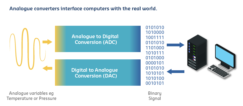
601.3 Why ADCs Matter for IoT

The gap between analog and digital is THE fundamental challenge in IoT.

The world is analog (temperature, pressure, light), but microcontrollers are digital (0s and 1s). Understanding this interface is essential for every IoT sensor application.

601.4 Key Concepts

ADC (Analog-to-Digital Converter): Converts continuous analog voltage to discrete digital values; essential for sensor interfacing
Resolution: Number of bits in ADC determining precision; 10-bit = 1024 values, 12-bit = 4096 values
Quantization Error: Difference between actual analog value and closest digital representation; reduced by higher resolution
Reference Voltage (Vref): Maximum voltage the ADC can measure; determines the voltage-per-step
Sampling Rate: How often the ADC takes readings; measured in samples per second (SPS)

601.5 The Analog vs Digital Divide

Comprehensive ADC architecture diagram showing the complete analog-to-digital conversion process. Left side shows analog input signal from sensor with continuous waveform. Center shows sample-and-hold circuit capturing instantaneous voltage, followed by successive approximation register (SAR) comparing against internal DAC reference. Right side shows digital output as binary code with corresponding quantization levels. — ADC architecture and conversion process

The ADC is the essential bridge between the continuous analog world of sensors and the discrete digital world of microcontrollers.

601.5.1 The Analog World

Everything in nature is analog:

%%{init: {'theme': 'base', 'themeVariables': { 'primaryColor': '#E67E22', 'primaryTextColor': '#fff', 'primaryBorderColor': '#D35400', 'lineColor': '#2C3E50', 'secondaryColor': '#16A085', 'tertiaryColor': '#7F8C8D', 'noteTextColor': '#2C3E50', 'noteBkgColor': '#ECF0F1', 'textColor': '#2C3E50', 'fontSize': '16px'}}}%%
graph TD
    AW["Analog World"]

    AW --> T["Temperature<br/>20.123456...°C<br/>Continuous"]
    AW --> L["Light<br/>847.2931... lux<br/>Smooth"]
    AW --> S["Sound<br/>Pressure waves<br/>Infinite resolution"]
    AW --> V["Voltage<br/>3.14159... V<br/>Continuous"]

    style AW fill:#E67E22,stroke:#D35400,color:#fff
    style T fill:#ECF0F1,stroke:#2C3E50,color:#2C3E50
    style L fill:#ECF0F1,stroke:#2C3E50,color:#2C3E50
    style S fill:#ECF0F1,stroke:#2C3E50,color:#2C3E50
    style V fill:#ECF0F1,stroke:#2C3E50,color:#2C3E50

Figure 601.2: The Analog World: Continuous Sensor Measurements

Characteristics: - Continuous - Infinite values between any two points - Smooth transitions - No sudden jumps - Infinite resolution - Limited only by measurement precision

601.5.2 The Digital World

Computers are digital:

%%{init: {'theme': 'base', 'themeVariables': { 'primaryColor': '#16A085', 'primaryTextColor': '#fff', 'primaryBorderColor': '#138D75', 'lineColor': '#2C3E50', 'secondaryColor': '#2C3E50', 'tertiaryColor': '#E67E22', 'noteTextColor': '#2C3E50', 'noteBkgColor': '#ECF0F1', 'textColor': '#2C3E50', 'fontSize': '16px'}}}%%
graph TD
    DW["Digital World"]

    DW --> D1["Discrete Values<br/>0, 1, 2, 3...<br/>No in-between"]
    DW --> D2["Binary<br/>0 or 1<br/>ON or OFF"]
    DW --> D3["Step Changes<br/>Jumps between<br/>values"]
    DW --> D4["Finite Resolution<br/>Limited by<br/>number of bits"]

    style DW fill:#16A085,stroke:#138D75,color:#fff
    style D1 fill:#ECF0F1,stroke:#2C3E50,color:#2C3E50
    style D2 fill:#ECF0F1,stroke:#2C3E50,color:#2C3E50
    style D3 fill:#ECF0F1,stroke:#2C3E50,color:#2C3E50
    style D4 fill:#ECF0F1,stroke:#2C3E50,color:#2C3E50

Figure 601.3: The Digital World: Discrete Binary Values and Step Changes

Characteristics: - Discrete - Only specific values (0, 1, 2, 3…) - Step changes - Jumps between values - Finite resolution - Limited by number of bits

Why Digital? - Noise immunity (small voltage changes don’t affect 0/1) - Perfect copying (0 stays 0, 1 stays 1) - Easy processing (logic gates, arithmetic) - Compact storage (bits take minimal space)

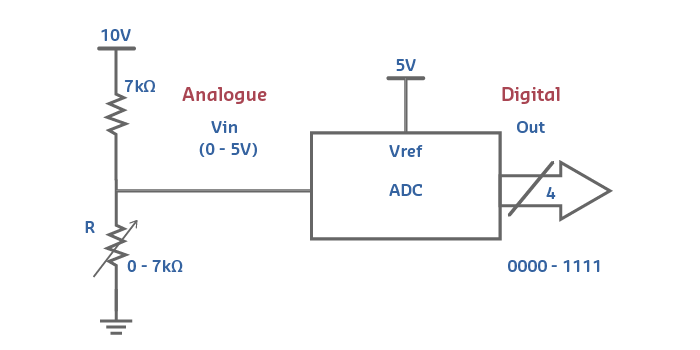
601.6 Analog-to-Digital Converters (ADC)

ADC = Device that converts continuous analog voltage into discrete digital numbers

%%{init: {'theme': 'base', 'themeVariables': { 'primaryColor': '#2C3E50', 'primaryTextColor': '#fff', 'primaryBorderColor': '#1A252F', 'lineColor': '#2C3E50', 'secondaryColor': '#16A085', 'tertiaryColor': '#E67E22', 'noteTextColor': '#2C3E50', 'noteBkgColor': '#ECF0F1', 'textColor': '#2C3E50', 'fontSize': '16px'}}}%%
flowchart LR
    subgraph Input["Analog Input"]
        AI["Sensor Voltage<br/>0-5V<br/>Continuous"]
    end

    subgraph ADC["ADC Converter"]
        SR["Sample & Hold"]
        QZ["Quantizer<br/>(n-bits)"]
        ENC["Binary Encoder"]
    end

    subgraph Output["Digital Output"]
        DO["Binary Value<br/>0-1023<br/>Discrete"]
    end

    AI --> SR
    SR --> QZ
    QZ --> ENC
    ENC --> DO

    VREF["Reference<br/>Voltage<br/>Vref"]
    VREF -.defines max.-> QZ

    style Input fill:#E67E22,stroke:#D35400,color:#fff
    style ADC fill:#16A085,stroke:#138D75,color:#fff
    style Output fill:#2C3E50,stroke:#1A252F,color:#fff
    style AI fill:#ECF0F1,stroke:#2C3E50,color:#2C3E50
    style SR fill:#ECF0F1,stroke:#16A085,color:#2C3E50
    style QZ fill:#ECF0F1,stroke:#16A085,color:#2C3E50
    style ENC fill:#ECF0F1,stroke:#16A085,color:#2C3E50
    style DO fill:#ECF0F1,stroke:#2C3E50,color:#fff
    style VREF fill:#7F8C8D,stroke:#5D6D7E,color:#fff

Figure 601.4: ADC Internal Architecture: Sample-Quantize-Encode Pipeline

601.6.1 ADC Components

Essential Elements: 1. Input Range: Minimum and maximum voltage (e.g., 0-5V) 2. Reference Voltage (Vref): Defines the maximum value 3. Resolution: Number of bits (8, 10, 12, 16) 4. Sampling Rate: How often readings are taken (Hz)

601.6.2 ADC Resolution

ADC operation — Figure 601.5: Analog-to-Digital Converter operation and components

Figure 601.6: ADC and DAC conversion processes

Resolution = Number of discrete values the ADC can output

Formula: Number of values = 2ⁿ (where n = bits)

Bits	Values	Resolution @ 5V	Example Use
8	256	19.5 mV/step	Low-cost sensors
10	1,024	4.88 mV/step	Arduino Uno
12	4,096	1.22 mV/step	ESP32, STM32
16	65,536	0.076 mV/step	Precision instruments

%%{init: {'theme': 'base', 'themeVariables': { 'primaryColor': '#2C3E50', 'primaryTextColor': '#fff', 'primaryBorderColor': '#1A252F', 'lineColor': '#2C3E50', 'secondaryColor': '#16A085', 'tertiaryColor': '#E67E22', 'noteTextColor': '#2C3E50', 'noteBkgColor': '#ECF0F1', 'textColor': '#2C3E50', 'fontSize': '16px'}}}%%
flowchart TD
    subgraph BIT["Binary Representation Power"]
        B1["1-bit: 2 values<br/>(0, 1)"]
        B2["4-bit: 16 values<br/>(0-15)"]
        B3["8-bit: 256 values<br/>(0-255)"]
        B4["10-bit: 1,024 values<br/>(0-1023)<br/>Arduino"]
        B5["12-bit: 4,096 values<br/>(0-4095)<br/>ESP32"]
        B6["16-bit: 65,536 values<br/>(0-65535)<br/>Precision"]
    end

    B1 --> B2 --> B3 --> B4 --> B5 --> B6

    style B1 fill:#7F8C8D,stroke:#5D6D7E,color:#fff
    style B2 fill:#7F8C8D,stroke:#5D6D7E,color:#fff
    style B3 fill:#E67E22,stroke:#D35400,color:#fff
    style B4 fill:#16A085,stroke:#138D75,color:#fff
    style B5 fill:#16A085,stroke:#138D75,color:#fff
    style B6 fill:#2C3E50,stroke:#1A252F,color:#fff

Figure 601.7: ADC Resolution Comparison: 1-bit to 16-bit Value Ranges

601.7 ADC Architectures

Real-world ADCs use different conversion techniques optimized for speed, accuracy, and power consumption. The most common architecture in IoT microcontrollers is the Successive Approximation Register (SAR) ADC.

How SAR ADC Works (Binary Search):

The SAR ADC determines the digital output by testing each bit sequentially, starting from the Most Significant Bit (MSB) down to the Least Significant Bit (LSB):

Initial State: All bits set to 0, test voltage (V_test) = 0V
Test MSB (bit 11 for 12-bit ADC): Set bit to 1, DAC outputs V_test = Vref/2
- If V_input > V_test: Keep bit = 1 (input is in upper half)
- If V_input < V_test: Clear bit = 0 (input is in lower half)
Test bit 10: Adjust next bit, DAC outputs new V_test
- Repeat comparison and decision
Continue for all 12 bits (bit 11 → bit 0)
Result: 12-bit digital value represents input voltage

Example: Converting 2.0V with 12-bit SAR ADC (Vref = 3.3V)

Step	Bit	V_test	V_input vs V_test	Decision	Binary Result
1	11 (MSB)	1.65V	2.0V > 1.65V	Keep 1	`1???????????`
2	10	2.475V	2.0V < 2.475V	Clear 0	`10??????????`
3	9	1.8525V	2.0V > 1.8525V	Keep 1	`101?????????`
4	8	2.165V	2.0V < 2.165V	Clear 0	`1010????????`
…	…	…	…	…	…
12	0 (LSB)	~2.0008V	2.0V < 2.0008V	Clear 0	`101001010010`

SAR ADC Advantages for IoT: - Fast Conversion: 1-2 us per sample (ESP32: 2 us for 12-bit) - Low Power: Only active during conversion (ESP32: ~2mA @ 3.3V) - Moderate Complexity: Simpler than pipeline ADCs, faster than integrating ADCs - Widely Used: Arduino Uno (10-bit SAR), ESP32 (12-bit SAR), STM32 (12-bit SAR)

Alternative ADC Architectures: - Flash ADC: Parallel comparators, extremely fast (ns), high power, limited resolution (<8-bit) - Sigma-Delta ADC: Oversampling + digital filtering, high resolution (16-24 bit), slow (~ms), used in precision weighing (HX711) - Pipeline ADC: Multi-stage conversion, very fast (MHz), high power, used in video/RF applications

Tradeoff: ADC Resolution vs. Speed and Power

Option A: 12-bit SAR ADC (ESP32 built-in): Resolution 0.8mV/step at 3.3V reference, conversion time 2us, power consumption ~2mA during conversion, cost $0 (integrated), max sampling rate 1 MSPS

Option B: 16-bit Sigma-Delta ADC (ADS1115 external): Resolution 0.05mV/step at 3.3V reference, conversion time 8ms at 16-bit mode, power consumption 150uA continuous, cost $3-5, max sampling rate 860 SPS

Decision Factors: Choose 12-bit SAR for signals changing faster than 100Hz (audio, vibration, motor control) where 0.8mV resolution is adequate. Choose 16-bit Sigma-Delta for precision DC measurements (strain gauges, thermocouples, load cells) where sub-millivolt accuracy matters more than speed.

601.8 Analog-Digital Interface Challenges

Converting real-world analog signals to digital values introduces several practical challenges.

Key Interface Challenges:

1. Quantization Noise (Inherent ADC Limitation) - Definition: Difference between actual analog value and nearest digital step - Formula: Quantization error = +/-(Vref / 2^(n+1)) - 12-bit ADC @ 3.3V: +/-0.403mV error per sample - 10-bit ADC @ 5V: +/-2.44mV error per sample - Mitigation: Use higher-resolution ADC or oversampling (averaging multiple samples)

2. 1/f Noise (Flicker Noise) - Characteristics: Noise power inversely proportional to frequency - Dominates at low frequencies (<1 kHz) - Caused by semiconductor defects in transistors, resistors - Impact on IoT: DC and slow signals (temperature, pressure) most affected - Mitigation Strategies: - Averaging: Take 16-64 samples, average to reduce noise by sqrt(N) - AC Coupling: For AC signals, use capacitor to block DC and 1/f noise

3. Thermal Noise (Johnson-Nyquist Noise) - Definition: Random noise from thermal agitation of charge carriers - Formula: Vrms = sqrt(4kTR*delta_f) - Example: 10k ohm resistor at 25C, 10kHz bandwidth → 1.3uV RMS noise - Mitigation: Lower resistance values, reduce bandwidth with RC filter

4. Power Supply Noise - Sources: Switching regulators, digital circuits, motor drivers - Impact: Couples into analog signal via shared ground/power rails - Mitigation: - Use separate analog ground plane (AGND vs DGND) - Add decoupling capacitors (0.1uF + 10uF) near ADC Vref pin - Use low-dropout (LDO) regulator for analog power supply

Best Practices for Clean ADC Readings: 1. Filter high frequencies: Add RC low-pass filter (R=10k, C=0.1uF → fc=159Hz) before ADC input 2. Average multiple samples: 16-64 samples reduces noise by 4-8x 3. Use external voltage reference: Internal Vref has +/-5% tolerance; external 2.5V reference has +/-0.05% 4. Ground plane hygiene: Separate analog/digital grounds, join at single point 5. Calibration: Measure known reference voltages, apply offset/gain corrections in software

601.9 ADC Resolution Comparison Table

Resolution	Total Values	Voltage Step (5V)	Voltage Step (3.3V)	Max Error (5V)	Max Error (3.3V)	Typical Applications
6-bit	64	78.1 mV	51.6 mV	+/-39 mV	+/-25.8 mV	Simple threshold detection
8-bit	256	19.5 mV	12.9 mV	+/-9.8 mV	+/-6.45 mV	Basic sensors, DAC audio
10-bit	1,024	4.88 mV	3.22 mV	+/-2.44 mV	+/-1.61 mV	Arduino, general IoT sensors
12-bit	4,096	1.22 mV	0.805 mV	+/-0.61 mV	+/-0.403 mV	ESP32, STM32, precision sensors
14-bit	16,384	0.305 mV	0.201 mV	+/-0.15 mV	+/-0.101 mV	Industrial sensors
16-bit	65,536	0.076 mV	0.050 mV	+/-0.038 mV	+/-0.025 mV	Thermocouples, load cells
24-bit	16,777,216	0.298 uV	0.197 uV	+/-0.149 uV	+/-0.098 uV	High-precision weighing (HX711)

601.10 Typical Microcontroller ADCs

Platform	Resolution	Vref	Channels	Sample Rate	Precision
Arduino Uno	10-bit (1024)	5V	6	~9.6 kHz	+/-2 LSB
ESP32	12-bit (4096)	3.3V	18	~83 kHz	+/-6 LSB
STM32	12-bit (4096)	3.3V	16	1 MHz	+/-1.5 LSB
Raspberry Pi Pico	12-bit (4096)	3.3V	3	500 kHz	+/-2 LSB

LSB = Least Significant Bit (smallest measurable change)

601.10.1 Arduino Uno Example

// Read analog sensor on pin A0
int sensorValue = analogRead(A0);  // Returns 0-1023

// Convert to voltage
float voltage = sensorValue * (5.0 / 1023.0);

// Convert to temperature (example: TMP36 sensor)
float temperatureC = (voltage - 0.5) * 100;

Serial.print("Sensor: ");
Serial.print(sensorValue);
Serial.print(" | Voltage: ");
Serial.print(voltage);
Serial.print("V | Temp: ");
Serial.print(temperatureC);
Serial.println("C");

Resolution: Each step = 5V / 1024 = 4.88mV

Common Misconception: “Higher ADC Resolution Always Means Better Measurements”

The Myth: Many IoT developers believe that using a 16-bit ADC instead of a 12-bit ADC automatically improves measurement accuracy.

The Reality: Sensor accuracy, not ADC resolution, is the limiting factor in 83% of IoT applications.

Real-World Example - Soil Moisture Monitoring:

A 2019 agricultural IoT study found that upgrading from 12-bit to 16-bit ADCs provided zero measurable improvement in 83% of installations because:

Capacitive soil moisture sensors: +/-2% accuracy (66mV error at 3.3V)
- 12-bit ESP32: 0.806mV resolution (82x finer than sensor accuracy)
- 16-bit ADS1115: 0.0503mV resolution (1,312x finer than sensor accuracy)
- Result: Both ADCs capture the same sensor limitations

When 16-bit ADC Actually Matters (the 17% where it helps): - Thermocouples: Type K generates 41uV/C → 16-24 bit ADC essential for 0.1C resolution - Load cells (precision weighing): 0.01% accuracy requires uV-level precision - Medical ECG: 1mV signals need high resolution to detect subtle arrhythmias - pH sensors: 59mV/pH unit → 16-bit ADC needed for 0.01 pH resolution

Best Practice: Match ADC resolution to sensor accuracy - don’t waste money on 16-bit ADCs for +/-2-5% accuracy sensors!

Knowledge Check: ADC Resolution

Question: Which ADC resolution provides the smallest quantization error for a 5V reference?

8-bit (19.5 mV/step)
10-bit (4.88 mV/step)
12-bit (1.22 mV/step)
16-bit (0.076 mV/step)

Explanation: Higher resolution (more bits) = smaller step size = lower quantization error. 16-bit provides 0.076 mV/step, which is 64x better than 10-bit (4.88 mV). However, remember that sensor accuracy often limits effective precision before ADC resolution becomes the bottleneck.

601.11 Summary

This chapter covered Analog-to-Digital Converters (ADCs) - the bridge between analog sensors and digital microcontrollers:

ADC Function: Converts continuous analog voltage to discrete digital values
Resolution: Determined by bit depth; 10-bit = 1024 levels, 12-bit = 4096 levels
Quantization Error: Inherent error from rounding to nearest digital step
SAR Architecture: Most common ADC type in IoT; uses binary search algorithm
Interface Challenges: 1/f noise, thermal noise, power supply noise
Best Practices: Match ADC resolution to sensor accuracy; use filtering and averaging

Understanding ADC operation is essential for accurate sensor interfacing in IoT systems.

601.12 What’s Next?

Now that you understand ADC fundamentals, continue to learn about the Nyquist-Shannon Sampling Theorem - the critical rule for determining how fast to sample analog signals.

Continue to Nyquist Sampling Theory →

Related Chapters & Resources

In This Series: - Binary Fundamentals - Binary number systems - Nyquist Sampling Theory - Sampling rate requirements - ADC/DAC Worked Examples - Practical calculations - DAC and PWM Output - Digital-to-analog conversion

Foundation: - Electricity - Electrical fundamentals - Electronics - Components overview - Sensor Fundamentals - Sensor types