1055 LPWAN Fundamentals: Pitfalls and Summary
This chapter connects to multiple learning resources across the book:
Interactive Tools: - Simulations Hub - Use the Interactive Range Calculator to experiment with link budget calculations for LoRa, Sigfox, and NB-IoT, exploring how TX power, antenna gain, and environment affect range estimates - Network Topology Visualizer - Explore how LPWAN gateways create star topology networks connecting thousands of end devices
Knowledge Checks: - Quiz Navigator - Test your LPWAN knowledge with technology selection scenarios, cost analysis problems, and deployment decision quizzes - Knowledge Gaps - Common misconceptions about LPWAN range, battery life, and reliability
Video Learning: - Videos Hub - Watch LoRaWAN architecture tutorials, Sigfox vs NB-IoT comparisons, and real-world smart city deployments
Knowledge Map: - Knowledge Map - See how LPWAN fundamentals connect to specific technologies (LoRaWAN, Sigfox, NB-IoT), WSN architectures, and IoT application domains
The Misconception: Many assume all LPWAN devices automatically achieve 5-10 year battery life regardless of configuration.
The Reality: Battery life depends critically on message frequency and payload size. Here’s quantified data:
LoRaWAN Battery Life Calculator (2,000 mAh battery, 3.6V):
| Messages/Day | Payload | SF | Battery Life | Why? |
|---|---|---|---|---|
| 1 msg/day | 12 bytes | SF12 | 10+ years | Optimal: infrequent, efficient |
| 24 msgs/day (hourly) | 50 bytes | SF7 | 5-7 years | Still good: reasonable frequency |
| 288 msgs/day (5 min) | 100 bytes | SF7 | 6-12 months | Power-hungry: constant TX |
| 1440 msgs/day (1 min) | 200 bytes | SF7 | 2-4 months | Unsustainable: LPWAN misuse |
Real-World Example - Smart Water Meter Project Failure:
A utility company deployed 10,000 LoRaWAN water meters expecting 10-year battery life. After 8 months, 30% of devices went offline.
Root cause analysis:
Expected configuration:
- 1 reading/day (365 msgs/year)
- 12-byte payload (meter ID + reading)
- SF12 for maximum range
- Predicted battery life: 10 years ✓

Actual configuration (implementation bug):
- 24 readings/day (8,760 msgs/year) - 24× more frequent!
- 243-byte payload (full JSON with metadata) - 20× larger!
- SF7 (weak signal forced SF12 retries)
- Actual battery life: 8-10 months ❌

Cost impact:
- Battery replacement: €25/device × 10,000 = €250,000
- Truck roll costs: €50/site × 10,000 = €500,000
- Total unplanned cost: €750,000
Key Lessons:
- Message frequency is exponential: 24× more messages = 20× shorter battery life due to radio warmup overhead
- Payload efficiency matters: Sending 243 bytes vs 12 bytes quadruples energy per transmission
- Spreading Factor impacts energy: SF12 uses 6× more energy than SF7 (longer TX time)
- Real range vs theoretical range: Poor gateway placement forced devices to use SF12, further draining batteries
How to Achieve Advertised Battery Life:
✅ Do: - Send ≤ 10 messages/day for 5+ year life - Use smallest payload possible (12-50 bytes) - Optimize gateway placement for SF7-SF9 - Measure actual current consumption in pilot
❌ Don’t: - Send messages every minute (LPWAN is not for real-time!) - Send JSON when binary encoding works - Assume poor coverage will be “fine” - Skip battery life calculations before deployment
Formula (simplified):
Battery Life (years) ≈ (Battery Capacity × 0.8) / (TX Current × TX Time × Messages/Day × 365)

Example (good design):
= (2000 mAh × 0.8) / (40 mA × 2 sec × 1 msg/day × 365)
= 1600 mAh / 29.2 mAh/year
≈ 55 years (capped by battery shelf life ~10 years)

Example (bad design - 5 min intervals):
= (2000 mAh × 0.8) / (40 mA × 2 sec × 288 msgs/day × 365)
= 1600 mAh / 8410 mAh/year
≈ 0.19 years = 2.3 months ❌
Takeaway: LPWAN’s multi-year battery life is conditional, not guaranteed. Always validate your application’s message pattern against actual power consumption measurements.
1055.1 Visual Reference Gallery
Explore these AI-generated diagrams that visualize LPWAN fundamental concepts:

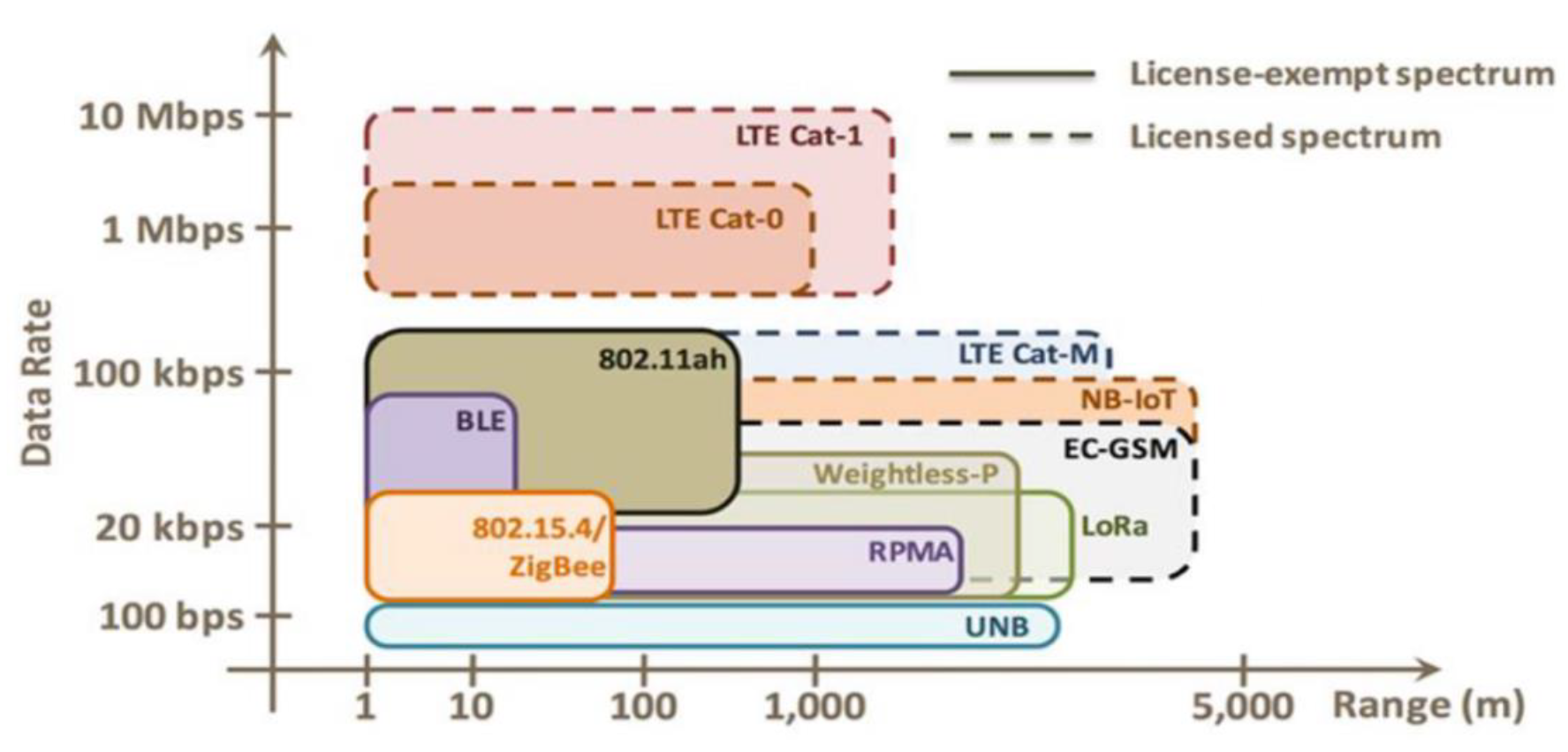
This diagram illustrates how different LPWAN technologies position themselves in the IoT connectivity spectrum, filling the gap between short-range Wi-Fi/Bluetooth and traditional cellular networks.

Understanding spreading factors is key to LoRaWAN deployment: higher SF provides longer range but slower data rates and increased power consumption.

LoRa uses Chirp Spread Spectrum (CSS) modulation to achieve remarkable receiver sensitivity (-137 dBm), enabling long-range communication in the unlicensed ISM bands.
1055.2 Summary
This chapter covered LPWAN fundamentals and technology characteristics:
- LPWAN Definition: Wireless communication protocols optimized for long-range (2-15 km urban, 40+ km rural), low-power (5-10 year battery life), and low-data-rate (hundreds of bps to few kbps) IoT applications
- Technology Positioning: LPWAN bridges the gap between short-range technologies and cellular networks in the IoT connectivity landscape
- Key Protocols: LoRaWAN (private networks), Sigfox (operator service), and NB-IoT/LTE-M (cellular LPWAN) represent different deployment and cost models
- Design Trade-offs: LPWAN technologies balance range, power consumption, data rate, and reliability based on application requirements
- Deployment Models: Private infrastructure (LoRaWAN) provides control and no subscription costs, while operator models (Sigfox, NB-IoT) offer managed coverage
- Reliability Characteristics: Different LPWAN technologies achieve varying reliability levels, from 85-95% (unconfirmed LoRaWAN) to 99.9%+ (NB-IoT with retransmission)
- Application Fit: LPWAN excels for infrequent, small-payload sensor updates but struggles with sub-minute intervals or high-data-rate applications
LPWAN Technologies: - LoRaWAN Overview - LoRa technology - Sigfox - Ultra-narrow band - NB-IoT - Cellular LPWAN - LPWAN Comparison - Technology comparison
Architecture: - WSN Overview - Sensor networks - Edge Fog Computing - Network tiers
IoT Products:
Interactive Tools: - Simulations Hub - Range calculator
Learning Hubs: - Quiz Navigator - LPWAN quizzes
These figures from the CP IoT System Design Guide provide alternative visual perspectives on LPWAN concepts covered in this chapter.
1055.2.1 LPWAN Technology Landscape
Source: CP IoT System Design Guide, Chapter 4 - LPWAN Protocols
1055.2.2 LoRaWAN Protocol Stack
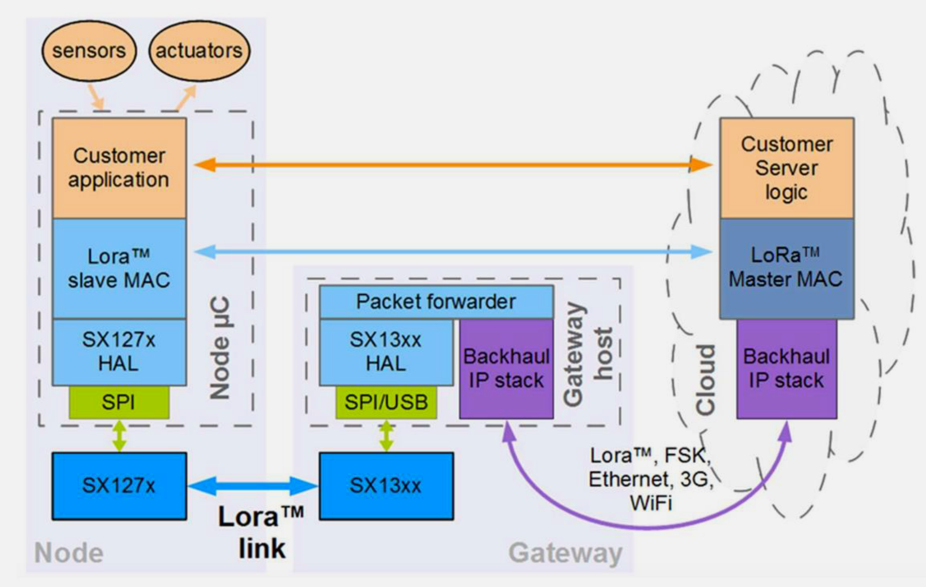
Source: CP IoT System Design Guide, Chapter 4 - LPWAN Protocols
1055.2.3 Sigfox Architecture
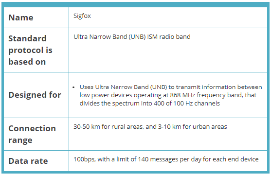
Source: CP IoT System Design Guide, Chapter 4 - LPWAN Protocols
1055.2.4 NB-IoT Paradigm
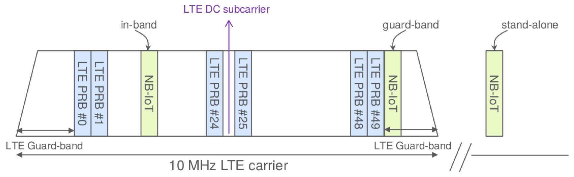
Source: CP IoT System Design Guide, Chapter 4 - LPWAN Protocols
1055.3 Common Pitfalls
The Mistake: Developers design applications that transmit too frequently without calculating time-on-air, leading to duty cycle violations. The device either silently drops messages (causing data loss) or violates regulations (risking fines and interference with other users).
Why It Happens: The EU868 band enforces a strict 1% duty cycle per sub-band. This means a device can transmit for a maximum of 36 seconds per hour per sub-band. Developers often calculate message frequency without considering spreading factor’s impact on airtime:
| SF | 20-byte ToA | Max msgs/hr (1%) | Common mistake |
|---|---|---|---|
| SF7 | 56 ms | 643 messages | “I can send every 5 seconds” - Wrong! |
| SF9 | 185 ms | 194 messages | “Hourly updates are fine” - Usually OK |
| SF12 | 1318 ms | 27 messages | “Every 2 minutes” - Violation! |
A developer sending 50-byte payloads every 5 minutes at SF12 (ToA ~2.5 seconds) accumulates 30 seconds of airtime per hour - seemingly within 1%. But if the device also sends join requests, confirmed uplinks with retries, or MAC commands, total airtime easily exceeds the limit.
The Fix: Calculate duty cycle budget precisely and monitor usage:
Calculate ToA accurately: Use the formula
ToA = (8 + max(ceil((8*PL - 4*SF + 28 + 16 - 20*H) / (4*(SF-2*DE))), 0) * (CR+4)) * Ts + TpreambleOr use online calculators: LoRa Airtime CalculatorBudget all transmissions:
Example budget (SF10, 125 kHz, 1 hr):
- 24 sensor readings (50 bytes): 24 x 370 ms = 8.9 sec
- 2 confirmed uplinks (ACK retry): 2 x 2 x 370 ms = 1.5 sec
- 1 join request (worst case): 1 x 1318 ms = 1.3 sec
- MAC command responses: ~0.5 sec
Total: 12.2 seconds (34% of 36-sec budget) - Safe
Implement airtime tracking: Store cumulative airtime per sub-band and block transmission if approaching limit
Use multiple sub-bands: EU868 has 8 channels across different sub-bands. Spread transmissions to multiply your effective budget
Regulatory consequences: Violations can result in fines up to 10,000 EUR in EU countries. More practically, excessive airtime causes collisions affecting all nearby LoRaWAN devices.
The Mistake: Developers assume duty cycle applies per-channel and freely hop between channels, not realizing that EU868 regulations aggregate duty cycle across entire sub-bands. A device hopping across 8 channels in the same sub-band still counts all airtime against a single 1% limit.
Why It Happens: LoRaWAN uses channel hopping to spread interference and improve reliability. Developers see 8 default channels (868.1, 868.3, 868.5 MHz in g1, plus others) and assume:
- “Each channel has its own 1% limit” - Wrong!
- “Hopping between channels resets my duty cycle” - Wrong!
- “I can send 8x more by using all channels” - Wrong!
EU868 sub-band structure:
Sub-band g  (863.0-865.0 MHz): 1.0% duty cycle - Includes 863.x channels
Sub-band g1 (865.0-868.0 MHz): 1.0% duty cycle - Includes 868.1/868.3/868.5
Sub-band g2 (868.0-868.6 MHz): 1.0% duty cycle - Overlaps with g1!
Sub-band g3 (868.7-869.2 MHz): 0.1% duty cycle - Very limited!
Sub-band g4 (869.4-869.65 MHz): 10% duty cycle - Best for downlinks
The three most common LoRaWAN channels (868.1, 868.3, 868.5 MHz) all fall within g1 sub-band. Hopping between them provides NO additional duty cycle budget.
The Fix: Design for sub-band, not channel, duty cycle:
- Map your channels to sub-bands: Know which sub-band each channel belongs to
- Track airtime per sub-band: Even with channel hopping, sum all transmissions in same sub-band
- Use channels in different sub-bands: Configure device to use channels across g1 AND g2 AND g4 (if gateway supports)
- Leverage g4 for downlinks: The 10% duty cycle sub-band (869.525 MHz) is ideal for gateway-to-device communication
Correct duty cycle calculation:
Device uses channels 868.1, 868.3, 868.5 (all in g1):
- 10 messages on 868.1: 10 x 200 ms = 2 sec
- 10 messages on 868.3: 10 x 200 ms = 2 sec
- 10 messages on 868.5: 10 x 200 ms = 2 sec
Total g1 airtime: 6 seconds (NOT 2 seconds per channel!)
g1 limit: 36 seconds/hour
Status: 16.7% of budget used (OK)

If developer thought per-channel: "Only 5.6% used" - Dangerous underestimate!
US915 has different rules (no duty cycle, but dwell time limits). Always verify regional parameters.
The Mistake: Developers build and test LPWAN applications using US915 frequencies (which have no duty cycle restrictions), then deploy in Europe where EU868’s strict 1% duty cycle causes message drops, join failures, and regulatory violations.
Why It Happens: The US915 and EU868 bands have fundamentally different regulatory constraints:
| Parameter | US915 | EU868 |
|---|---|---|
| Duty cycle | None (FCC Part 15) | 1% per sub-band (ETSI EN 300.220) |
| Max TX time/hour | Unlimited | 36 seconds (1% of 3600s) |
| Dwell time limit | 400ms (frequency hopping) | None |
| Channels | 64 uplink + 8 downlink | 8-16 typical |
A device sending 20-byte payloads every 2 minutes works perfectly on US915:
US915: 30 msgs/hour × any SF = OK (no limit)
EU868 SF10: 30 msgs/hour × 370ms = 11.1 sec (OK, 31% of budget)
EU868 SF12: 30 msgs/hour × 1318ms = 39.5 sec (VIOLATION! 110% of budget)
The Fix: Design for the most restrictive region (EU868) first:
- Calculate worst-case airtime: Use SF12 ToA for capacity planning, even if ADR will optimize
- Budget for all transmissions: Include joins, retries, MAC commands, not just data uplinks
- Test with duty cycle enforcement: Enable LMIC_setClockError() or equivalent to simulate regulatory limits
- Implement airtime tracking: Maintain per-sub-band counters and block TX when approaching limits
EU868 transmission budget calculator:
Hourly budget: 36,000 ms (1% of 3,600,000 ms)

SF7 (56ms/msg): 643 messages/hour max
SF9 (185ms/msg): 194 messages/hour max
SF10 (370ms/msg): 97 messages/hour max
SF12 (1318ms/msg): 27 messages/hour max

Safe design rule: Plan for 50% of budget to handle retries
SF10 practical limit: ~48 msgs/hour
SF12 practical limit: ~13 msgs/hour
Multi-region deployment strategy: Use ADR aggressively in EU868 (lower SF = more messages allowed), configure region-specific transmission intervals, and implement graceful degradation when duty cycle budget is exhausted.
The Mistake: Developers select spreading factor solely based on required range (e.g., “I need 10 km, so I’ll use SF12”), ignoring that higher SF dramatically reduces network capacity and increases collision probability in shared deployments.
Why It Happens: Range-focused selection ignores the network-level impact of spreading factor:
- SF selection charts typically show only range, not capacity
- Single-device testing doesn’t reveal multi-device collision rates
- Gateway capacity depends on total airtime, not message count
- Collision probability scales with time-on-air (longer packets more likely to overlap)
Network capacity comparison for single 8-channel gateway:
| SF | ToA (20 bytes) | Capacity/channel/hour | Total gateway capacity | Collision rate (100 devices) |
|---|---|---|---|---|
| SF7 | 56ms | 643 msgs | ~5,000 msgs/hr | 0.3% |
| SF9 | 185ms | 194 msgs | ~1,500 msgs/hr | 1.1% |
| SF10 | 370ms | 97 msgs | ~750 msgs/hr | 2.2% |
| SF12 | 1318ms | 27 msgs | ~216 msgs/hr | 7.8% |
A 100-device network sending every 10 minutes (600 msgs/hour): - At SF7: 12% gateway utilization, <1% collisions - At SF10: 80% gateway utilization, 3-5% collisions - At SF12: 278% utilization - NETWORK COLLAPSE (messages dropped)
The Fix: Balance range against capacity using ADR and network planning:
- Enable ADR: Let network server optimize SF per device based on actual link quality
- Plan for SF distribution: Assume 30% SF7-8, 40% SF9-10, 30% SF11-12 in typical deployments
- Add gateways for capacity, not just coverage: One gateway covers 10km range but may only support 200 devices at SF12
- Use link budget, not distance: Calculate required SF from TX power, antenna gains, path loss, and fade margin
Capacity planning formula:
Required SF = ceiling(log2(Link_Budget_dB / 3) + 7)
Where Link_Budget_dB = TX_Power + TX_Antenna + RX_Antenna - Path_Loss - Fade_Margin - RX_Sensitivity

Example: 5km urban deployment
TX Power: 14 dBm
Antennas: +2 dBi each
Path Loss: 120 dB (urban 868 MHz)
Fade Margin: 10 dB
RX Sensitivity: -137 dBm (SF12)

Link Budget: 14 + 2 + 2 - 120 - 10 - (-137) = 25 dB margin
Required SF: ceil(log2(25/3) + 7) = ceil(10.1) = SF11 (minimum)

ADR will likely optimize to SF9 after 50 uplinks if actual margin > 20 dB
Rule of thumb: If more than 20% of devices need SF12, add another gateway rather than accepting reduced capacity.
1055.4 Key Takeaways
Core Concepts: - LPWAN technologies trade data rate for range and battery life: 2-15 km range, 5-10 year battery operation, but only hundreds of bps to few kbps - Three main approaches: LoRaWAN (private gateways, open standard), Sigfox (operator network, proprietary), NB-IoT/LTE-M (cellular infrastructure) - LPWAN fills the gap between short-range Wi-Fi/Bluetooth and expensive cellular, ideal for small-payload sensor applications - Deployment models determine control and cost: private infrastructure provides autonomy while operator models offer managed coverage
Practical Applications: - Smart agriculture: soil moisture sensors across 100 km² farms with multi-year battery life and hourly updates - Smart cities: parking sensors, waste bins, water meters sending small readings without cellular subscription costs - LoRaWAN becomes cost-effective after year 3 for 1,000 sensors (€17,500 total vs Sigfox’s €25,000 over 10 years) - Global logistics requires NB-IoT/LTE-M cellular for mobile asset tracking with worldwide carrier coverage
Design Considerations: - Choose NB-IoT for 99.9% reliability requirements (licensed spectrum, carrier SLA) vs LoRaWAN’s 85-95% unconfirmed delivery - Private LoRaWAN deployment suits rural areas without operator coverage and provides data privacy control - Sigfox’s 4 downlinks/day limitation makes it unsuitable for bidirectional control applications (streetlights, actuators) - Battery sensors should use CoAP over LPWAN rather than TCP/MQTT to avoid connection overhead
Common Pitfalls: - Expecting LPWAN to support video streaming or real-time interactive applications (data rate too low for high-bandwidth needs) - Deploying Sigfox without considering operator bankruptcy risk (single vendor dependency vs cellular’s carrier redundancy) - Assuming LoRaWAN works globally without infrastructure (requires gateway deployment at every coverage location) - Using LPWAN for applications requiring sub-minute latency (protocols optimized for infrequent updates, not instant response)
1055.5 What’s Next
The next chapter explores LPWAN Architectures, covering the network topologies, device classes, and infrastructure models used by different LPWAN technologies.