792 Wired Communication Fundamentals

792.1 Learning Objectives

By the end of this section, you will be able to:

Understand the Binary Transmission Challenge: Explain how digital data is converted to electrical signals
Compare Synchronous vs Asynchronous: Differentiate clock-shared and independent-clock communication
Identify Network Topologies: Distinguish point-to-point, multi-drop, and multi-point configurations
Explain Master-Slave Architecture: Describe how bus access is controlled to prevent collisions
Choose Duplex Mode: Select full-duplex or half-duplex based on application requirements

792.2 Prerequisites

Before diving into this chapter, you should be familiar with:

Networking Basics: Understanding fundamental networking concepts including data transmission, protocols, and communication models
Binary and Digital Logic: Understanding binary numbers, voltage levels (HIGH/LOW), and basic digital electronics

792.3 Getting Started (For Beginners)

What Are Wired Communication Protocols? (Simple Explanation)

Analogy: Wired protocols are like different languages for talking through wires.

Just like humans have different languages (English, Spanish, Mandarin), electronic devices have different “languages” for communicating through wires (I2C, SPI, UART).

%%{init: {'theme': 'base', 'themeVariables': { 'primaryColor': '#2C3E50', 'primaryTextColor': '#fff', 'primaryBorderColor': '#16A085', 'lineColor': '#16A085', 'secondaryColor': '#E67E22', 'tertiaryColor': '#7F8C8D', 'noteTextColor': '#2C3E50', 'noteBkgColor': '#E8F6F3', 'noteBorderColor': '#16A085'}}}%%
graph LR
    A["Microcontroller<br/>(ESP32)"]
    B["Sensor 1<br/>(Temperature)"]
    C["Display<br/>(OLED)"]
    D["Storage<br/>(SD Card)"]

    A -->|"UART<br/>(2 wires)"| B
    A -->|"I2C<br/>(2 wires)"| C
    A -->|"SPI<br/>(4+ wires)"| D

    style A fill:#2C3E50,stroke:#16A085,color:#fff
    style B fill:#16A085,stroke:#16A085,color:#fff
    style C fill:#16A085,stroke:#16A085,color:#fff
    style D fill:#16A085,stroke:#16A085,color:#fff

Figure 792.1: Microcontroller Peripheral Connections Using UART, I2C, and SPI

Why Wired Protocols?: Microcontrollers and sensors need a shared “language” (protocol) to communicate through wires.

The Three Main Protocols: Quick Comparison

Protocol	Wires Needed	Speed	Devices	Best For
UART	2 (TX, RX)	Slow-Medium	2 only	GPS, Bluetooth modules
I2C	2 (SDA, SCL)	Medium	Many (127)	Sensors, displays
SPI	4+ (MOSI, MISO, SCK, CS)	Fast	Many	SD cards, fast sensors

%%{init: {'theme': 'base', 'themeVariables': { 'primaryColor': '#2C3E50', 'primaryTextColor': '#fff', 'primaryBorderColor': '#16A085', 'lineColor': '#16A085', 'secondaryColor': '#E67E22', 'tertiaryColor': '#7F8C8D'}}}%%
graph TD
    subgraph "UART: Point-to-Point"
        U1["Device 1"]
        U2["Device 2"]
        U1 <-->|"TX/RX<br/>(2 wires)"| U2
    end

    subgraph "I2C: Multi-Drop Bus"
        M["Master"]
        S1["Slave 1"]
        S2["Slave 2"]
        S3["Slave 3"]
        M ---|"SDA/SCL<br/>(2 wires)"| S1
        M ---|"Shared Bus"| S2
        M ---|"Shared Bus"| S3
    end

    subgraph "SPI: Multi-Point Star"
        SP["Master"]
        SL1["Slave 1"]
        SL2["Slave 2"]
        SP -->|"MOSI/MISO/SCK/CS1<br/>(4 wires)"| SL1
        SP -->|"MOSI/MISO/SCK/CS2<br/>(5 wires)"| SL2
    end

    style U1 fill:#2C3E50,stroke:#16A085,color:#fff
    style U2 fill:#2C3E50,stroke:#16A085,color:#fff
    style M fill:#2C3E50,stroke:#16A085,color:#fff
    style S1 fill:#16A085,stroke:#16A085,color:#fff
    style S2 fill:#16A085,stroke:#16A085,color:#fff
    style S3 fill:#16A085,stroke:#16A085,color:#fff
    style SP fill:#2C3E50,stroke:#16A085,color:#fff
    style SL1 fill:#16A085,stroke:#16A085,color:#fff
    style SL2 fill:#16A085,stroke:#16A085,color:#fff

Figure 792.2: UART, I2C, and SPI Topology Comparison

Alternative View: Wired Protocol Speed vs Complexity Trade-off

This variant visualizes the fundamental trade-off between protocol speed and implementation complexity - useful for choosing the right protocol for your project.

%%{init: {'theme': 'base', 'themeVariables': {'primaryColor': '#2C3E50', 'primaryTextColor': '#fff', 'primaryBorderColor': '#16A085', 'lineColor': '#E67E22', 'secondaryColor': '#16A085', 'tertiaryColor': '#E8F6F3', 'fontSize': '10px'}}}%%
flowchart LR
    subgraph SIMPLE["Simple (Few Wires)"]
        UART["UART<br/>2 wires<br/>115 kbps typ<br/>Point-to-point"]
        I2C["I2C<br/>2 wires<br/>400 kbps typ<br/>Multi-device"]
    end

    subgraph COMPLEX["Complex (More Wires)"]
        SPI["SPI<br/>4+ wires<br/>10+ Mbps<br/>High speed"]
        QSPI["QSPI<br/>6 wires<br/>100+ Mbps<br/>Flash memory"]
    end

    UART -->|"Need more<br/>devices"| I2C
    I2C -->|"Need more<br/>speed"| SPI
    SPI -->|"Need max<br/>throughput"| QSPI

    style UART fill:#16A085,stroke:#2C3E50,color:#fff
    style I2C fill:#16A085,stroke:#2C3E50,color:#fff
    style SPI fill:#E67E22,stroke:#2C3E50,color:#fff
    style QSPI fill:#2C3E50,stroke:#16A085,color:#fff

Figure 792.3: Wired Protocol Speed vs Complexity - Each step right adds wires but increases speed

Key Insight: I2C is the “sweet spot” for most IoT sensor applications - minimal wires (2) with multi-device support. Only move to SPI when I2C’s ~400 kbps isn’t fast enough.

When to Use Which Protocol?

Scenario	Best Choice	Why
Connect a GPS module	UART	GPS modules typically use serial
Connect 5 sensors	I2C	One bus for many devices
Read an SD card	SPI	Needs high speed
Connect a display	I2C or SPI	Depends on display type

Rule of thumb:

I2C = Default choice for most sensors (simple, few wires)
SPI = When you need speed (SD cards, high-res displays)
UART = Legacy devices, GPS, Bluetooth modules

Why Wired Communication Matters for IoT

At the local level, IoT devices communicate using wires. Sensors connect to microcontrollers via I2C, SPI, or UART. Industrial equipment uses RS-232. Understanding these protocols is essential for interfacing sensors, displays, and peripherals in IoT systems.

792.4 The Challenge: Transmitting Binary Data

792.4.1 Fundamental Problem

All IoT ecosystems communicate using binary protocols - endless trails of 0s and 1s.

%%{init: {'theme': 'base', 'themeVariables': { 'primaryColor': '#2C3E50', 'primaryTextColor': '#fff', 'primaryBorderColor': '#16A085', 'lineColor': '#16A085', 'secondaryColor': '#E67E22'}}}%%
graph LR
    A["Data:<br/>Temperature = 25C"]
    B["Binary:<br/>00011001"]
    C["Signal:<br/>HIGH/LOW"]
    D["Received:<br/>00011001"]
    E["Data:<br/>25C"]

    A --> B --> C --> D --> E

    style A fill:#2C3E50,stroke:#16A085,color:#fff
    style B fill:#16A085,stroke:#16A085,color:#fff
    style C fill:#E67E22,stroke:#16A085,color:#fff
    style D fill:#16A085,stroke:#16A085,color:#fff
    style E fill:#2C3E50,stroke:#16A085,color:#fff

Figure 792.4: Serial Data Transmission from Sensor Reading to Digital Value

The problem to solve:

How can we send 0s and 1s from one place to another?

Engineers have developed many solutions, each optimized for different scenarios.

792.4.2 Design Considerations

Choice of protocol depends on:

Factor	Questions	Impact
Distance	Same PCB? Same room? Same building?	Wire length limits speed
Speed	How fast must data move?	Faster = more complex circuitry
Safety	Security requirements? Interference?	Shielding, encryption costs
Cost	Budget constraints?	More wires = higher cost
Power	Battery or mains powered?	Low power = slower speeds

792.5 Overview of Wired Communication Standards

792.5.1 Comparison Table

Protocol	Wires	Sync/Async	Speed	Distance	Devices	Topology	IoT Use Case
RS-232	3-9	Async	115 kbps	15m	2	Point-to-point	GPS modules, serial debugging
I2C	2	Sync	400 kbps	<1m	112	Multi-drop	Sensors, displays, EEPROMs
SPI	4+	Sync	10+ Mbps	<1m	Many	Multi-point	SD cards, displays, high-speed sensors

At local level (same room/building), wired communication is most common for IoT device interconnections.

Overview diagram of common wired communication protocols for IoT: UART for serial communication, I2C for multi-device bus, SPI for high-speed peripherals, RS-232/RS-485 for industrial, and Ethernet for networking — Figure 792.5: Common wired communication standards for IoT including UART, I2C, SPI, and Ethernet

Table 792.1

Table: Wired Communication Standards Comparison

NAME	SYNC/ASYNC	TYPE	DUPLEX	MAX DEVICES	MAX SPEED (Kbps)	MAX DISTANCE (m)	PIN COUNT
RS-232	async	point-to-point	full	2	20	30	2
RS-422	async	multi-drop	half	10	10,000	4,000	1
RS-485	async	multi-point	half	32	10,000	4,000	2
I2C	sync	multi-master	half	112	3,400	<1	2
SPI	sync	multi-master	full	Many	>1,000	<1	3+1
1-Wire	async	master/slave	half	Many	16	1,000	1
USB 2.0	async	master/slave	half	127	480,000	5	4
USB 3.0	async	master/slave	full	255	5,000,000	5	8

792.6 Common Misconception

“More Wires = Always Better Performance”

Misconception: “SPI is always faster than I2C because it uses more wires (4+ vs 2), so I should always choose SPI for better performance.”

Reality: While SPI can achieve higher speeds (10+ Mbps vs 400 kHz), the real-world performance difference is often negligible for most IoT applications:

Quantified Examples:

BME280 Temperature Sensor:
- I2C @ 400 kHz: Reading temp/humidity/pressure takes ~8 ms
- SPI @ 10 MHz: Same reading takes ~5 ms
- Difference: 3 ms savings (37% faster)
- Reality: For a weather station reading every 10 seconds, this 3 ms difference is irrelevant (0.03% of cycle time)
0.96” OLED Display (128x64 px):
- I2C @ 400 kHz: Full screen refresh ~60 ms
- SPI @ 8 MHz: Full screen refresh ~30 ms
- Difference: 30 ms savings (50% faster)
- Reality: Both achieve 15+ fps, imperceptible to human eye
SD Card Data Logging:
- I2C (not supported): N/A
- SPI @ 25 MHz: 512-byte sector write ~200 us
- Reality: Here SPI is essential not because of “more wires” but because SD cards don’t support I2C protocol

Why the misconception?

Pin count does not equal performance: I2C’s 2-wire limitation isn’t the bottleneck; it’s the pull-up resistor RC time constant (rise time limits frequency)
Protocol overhead: I2C has 7-bit addressing + ACK bits (9 bits per byte), while SPI has 8 bits per byte - but for multi-byte transfers, this overhead is ~10%
Real bottleneck: Sensor conversion time (BME280 takes 8 ms to measure, regardless of interface speed)

When SPI truly matters:

High-throughput: SD cards, high-resolution TFT displays (320x240+), camera modules
Continuous streaming: Audio I2S (2.8 Mbps for 44.1 kHz stereo), DMA-driven data acquisition
Low latency: Real-time motor control loops (<1 ms cycle time)

The trade-off: SPI saves 1-5 ms per transaction but costs 2-3 extra GPIO pins per device. For battery-powered IoT nodes with limited pins, I2C is often superior despite lower speed.

Alternative View: Wired Interface Selection Flowchart

This variant presents wired communication selection through a decision-tree lens - useful for IoT designers choosing between UART, I2C, SPI, and RS-485 for specific hardware requirements.

%%{init: {'theme': 'base', 'themeVariables': {'primaryColor': '#2C3E50', 'primaryTextColor': '#fff', 'primaryBorderColor': '#16A085', 'lineColor': '#E67E22', 'secondaryColor': '#16A085', 'tertiaryColor': '#7F8C8D', 'fontSize': '11px'}}}%%
flowchart TD
    START["Select Wired<br/>Interface"]

    Q1{"Distance<br/>requirement?"}
    Q2{"Multiple<br/>devices on<br/>same bus?"}
    Q3{"Speed<br/>requirement?"}
    Q4{"Pin count<br/>constraint?"}

    UART["UART/RS-232<br/>2-3 wires, 115 kbps<br/>Point-to-point<br/>Best for: GPS,<br/>debug console"]

    RS485["RS-485<br/>2 wires, 10 Mbps<br/>Multi-drop, 4000m<br/>Best for: Industrial,<br/>Modbus sensors"]

    I2C["I2C<br/>2 wires, 400 kbps<br/>112 devices, <1m<br/>Best for: Sensors,<br/>EEPROMs, RTCs"]

    SPI["SPI<br/>4+ wires, 10+ Mbps<br/>Fast transfers<br/>Best for: Displays,<br/>SD cards, ADCs"]

    START --> Q1
    Q1 -->|">10m"| RS485
    Q1 -->|"<10m"| Q2

    Q2 -->|"No<br/>(1 device)"| UART
    Q2 -->|"Yes"| Q3

    Q3 -->|">1 Mbps"| SPI
    Q3 -->|"<1 Mbps"| Q4

    Q4 -->|"Minimal<br/>(2 pins)"| I2C
    Q4 -->|"Available<br/>(4+ pins)"| SPI

    style START fill:#2C3E50,stroke:#16A085,color:#fff
    style Q1 fill:#16A085,stroke:#2C3E50,color:#fff
    style Q2 fill:#16A085,stroke:#2C3E50,color:#fff
    style Q3 fill:#16A085,stroke:#2C3E50,color:#fff
    style Q4 fill:#16A085,stroke:#2C3E50,color:#fff
    style UART fill:#E67E22,stroke:#2C3E50,color:#fff
    style RS485 fill:#E67E22,stroke:#2C3E50,color:#fff
    style I2C fill:#E67E22,stroke:#2C3E50,color:#fff
    style SPI fill:#E67E22,stroke:#2C3E50,color:#fff

Figure 792.6: Decision flowchart for selecting wired communication interface based on distance, device count, speed, and pin constraints

792.7 Key Concepts

Before diving into specific protocols, understand these fundamental concepts:

792.7.1 Protocol

Definition: A set of rules and conventions governing information exchange between devices.

Example: TCP/IP (seen in previous chapters) is a protocol suite for internet communication.

792.7.2 Synchronous vs Asynchronous Communication

%%{init: {'theme': 'base', 'themeVariables': { 'primaryColor': '#2C3E50', 'primaryTextColor': '#fff', 'primaryBorderColor': '#16A085', 'lineColor': '#16A085', 'secondaryColor': '#E67E22'}}}%%
graph TB
    subgraph "Synchronous (I2C, SPI)"
        S1["Device A"]
        S2["Device B"]
        SC["Shared Clock"]
        S1 -->|"Data"| S2
        SC -.->|"Clock Signal"| S1
        SC -.->|"Clock Signal"| S2
    end

    subgraph "Asynchronous (UART)"
        A1["Device C<br/>Own Clock"]
        A2["Device D<br/>Own Clock"]
        A1 <-->|"Data + Start/Stop Bits"| A2
    end

    style S1 fill:#2C3E50,stroke:#16A085,color:#fff
    style S2 fill:#2C3E50,stroke:#16A085,color:#fff
    style SC fill:#16A085,stroke:#16A085,color:#fff
    style A1 fill:#E67E22,stroke:#16A085,color:#fff
    style A2 fill:#E67E22,stroke:#16A085,color:#fff

Figure 792.7: Synchronous vs Asynchronous Communication Timing

Synchronous:

Devices share a common clock transmitted on a dedicated wire
Data synchronized to clock edges
Simpler, more reliable
Examples: I2C, SPI

Asynchronous:

No clock wire transmitted
Devices run independent clocks at same speed
Data lines used for synchronization (start/stop bits)
Example: RS-232, UART

792.7.3 Peer Communication

Definition: Entities at the same layer of a network that communicate with each other.

Peer-to-peer communication diagram showing two devices directly connected and communicating without intermediary, both acting as equals in bidirectional data exchange — Figure 792.8: Peer communication showing direct device-to-device connections

%%{init: {'theme': 'base', 'themeVariables': { 'primaryColor': '#2C3E50', 'primaryTextColor': '#fff', 'primaryBorderColor': '#16A085', 'lineColor': '#16A085', 'secondaryColor': '#E67E22'}}}%%
graph LR
    M["Master<br/>(Layer 2)"]
    S1["Slave 1<br/>(Layer 2)"]
    S2["Slave 2<br/>(Layer 2)"]

    M <-->|"Peer Communication"| S1
    M <-->|"Peer Communication"| S2

    style M fill:#2C3E50,stroke:#16A085,color:#fff
    style S1 fill:#16A085,stroke:#16A085,color:#fff
    style S2 fill:#16A085,stroke:#16A085,color:#fff

Figure 792.9: Master-Slave Peer Communication at Layer 2

In wired protocols: Master and slave are peers at the same protocol layer.

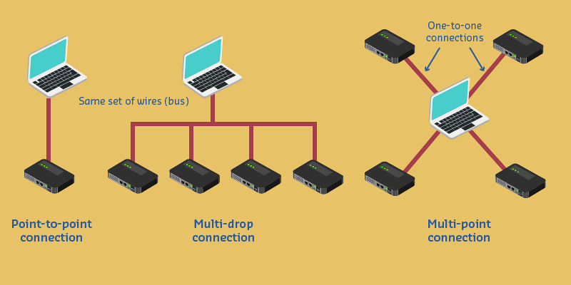
792.7.4 Point-to-Point, Multi-Drop, Multi-Point

Three connection topologies: point-to-point with single dedicated link between two devices, multi-drop with multiple devices on shared bus, and multi-point with selective device addressing — Figure 792.10: Point-to-point, multi-drop, and multi-point network topologies

%%{init: {'theme': 'base', 'themeVariables': { 'primaryColor': '#2C3E50', 'primaryTextColor': '#fff', 'primaryBorderColor': '#16A085', 'lineColor': '#16A085', 'secondaryColor': '#E67E22'}}}%%
graph TD
    subgraph "Point-to-Point (RS-232)"
        PP1["Device A"]
        PP2["Device B"]
        PP1 <-->|"Dedicated Wires"| PP2
    end

    subgraph "Multi-Drop (I2C)"
        MD["Master"]
        MDS1["Slave 1"]
        MDS2["Slave 2"]
        MDS3["Slave 3"]
        MD ---|"Shared Bus"| MDS1
        MD ---|"Shared Bus"| MDS2
        MD ---|"Shared Bus"| MDS3
    end

    subgraph "Multi-Point (SPI)"
        MP["Master"]
        MPS1["Slave 1"]
        MPS2["Slave 2"]
        MP -->|"CS1"| MPS1
        MP -->|"CS2"| MPS2
    end

    style PP1 fill:#2C3E50,stroke:#16A085,color:#fff
    style PP2 fill:#2C3E50,stroke:#16A085,color:#fff
    style MD fill:#2C3E50,stroke:#16A085,color:#fff
    style MDS1 fill:#16A085,stroke:#16A085,color:#fff
    style MDS2 fill:#16A085,stroke:#16A085,color:#fff
    style MDS3 fill:#16A085,stroke:#16A085,color:#fff
    style MP fill:#2C3E50,stroke:#16A085,color:#fff
    style MPS1 fill:#16A085,stroke:#16A085,color:#fff
    style MPS2 fill:#16A085,stroke:#16A085,color:#fff

Figure 792.11: Point-to-Point, Multi-Drop, and Multi-Point Topology Comparison

Point-to-Point:

Two devices using dedicated wires
Example: RS-232

Multi-Drop:

Many devices sharing same set of wires (bus)
Example: I2C

Multi-Point:

One master connecting to multiple slaves via dedicated wires
Example: SPI with multiple chip select lines

792.7.5 Master/Slave Networks

Master device:

Controls communication channel
Initiates all transactions
Determines when communication finishes

Slave devices:

Respond to master requests
Cannot talk directly to each other
Must wait for master to grant access

%%{init: {'theme': 'base', 'themeVariables': { 'primaryColor': '#2C3E50', 'primaryTextColor': '#fff', 'primaryBorderColor': '#16A085', 'lineColor': '#16A085', 'secondaryColor': '#E67E22'}}}%%
graph TB
    M["Master<br/>(Controls Bus)"]
    S1["Slave 1"]
    S2["Slave 2"]
    S3["Slave 3"]

    M -->|"1. Request"| S1
    S1 -->|"2. Response"| M
    M -->|"3. Request"| S2
    S2 -->|"4. Response"| M

    S1 -.-x|"Cannot talk directly"| S2
    S2 -.-x|"Cannot talk directly"| S3

    style M fill:#2C3E50,stroke:#16A085,color:#fff
    style S1 fill:#16A085,stroke:#16A085,color:#fff
    style S2 fill:#16A085,stroke:#16A085,color:#fff
    style S3 fill:#7F8C8D,stroke:#16A085,color:#fff

Figure 792.12: Master-Slave Communication Pattern with Collision Prevention

Prevents collisions: Only master controls when devices transmit.

792.7.6 Full-Duplex vs Half-Duplex

Full-Duplex:

Both endpoints can transmit simultaneously
Requires separate wires for each direction
Example: SPI (MOSI and MISO wires)

Half-Duplex:

Only one endpoint transmits at a time
Can share single wire (bidirectional)
Example: I2C (SDA line shared)

%%{init: {'theme': 'base', 'themeVariables': { 'primaryColor': '#2C3E50', 'primaryTextColor': '#fff', 'primaryBorderColor': '#16A085', 'lineColor': '#16A085', 'secondaryColor': '#E67E22'}}}%%
graph LR
    subgraph "Full-Duplex (SPI)"
        FD1["Device A"]
        FD2["Device B"]
        FD1 -->|"MOSI"| FD2
        FD2 -->|"MISO"| FD1
    end

    subgraph "Half-Duplex (I2C)"
        HD1["Device C"]
        HD2["Device D"]
        HD1 <-->|"SDA (Shared)"| HD2
    end

    style FD1 fill:#2C3E50,stroke:#16A085,color:#fff
    style FD2 fill:#2C3E50,stroke:#16A085,color:#fff
    style HD1 fill:#16A085,stroke:#16A085,color:#fff
    style HD2 fill:#16A085,stroke:#16A085,color:#fff

Figure 792.13: Full-Duplex vs Half-Duplex Communication Modes

792.8 Summary

This chapter introduced the fundamental concepts of wired communication:

Binary transmission challenge: Converting digital data to electrical signals requires standardized protocols
Synchronous vs asynchronous: Clock-shared protocols (I2C, SPI) are simpler; independent-clock protocols (UART) need start/stop bits
Network topologies: Point-to-point for dedicated links, multi-drop for shared buses, multi-point for star configurations
Master-slave architecture: Prevents collisions by having one device control bus access
Full vs half duplex: Trade-off between simultaneous bidirectional communication and wire count

792.9 What’s Next

Now that you understand wired communication fundamentals, explore the specific protocols:

UART and RS-232: Serial point-to-point communication for GPS and debugging
I2C Protocol: Two-wire bus for sensors, displays, and EEPROMs
SPI Protocol: High-speed interface for SD cards and fast peripherals