780  Network Topologies: Labs and Design

780.1 Learning Objectives

By the end of this chapter, you will be able to:

• Draw Network Diagrams: Create logical and physical topology diagrams using industry-standard tools
• Design Star Networks: Plan Wi-Fi-based IoT deployments with central access points
• Implement Mesh Topologies: Configure self-healing mesh networks using Zigbee or Thread
• Document Installations: Produce professional network documentation including floor plans and cable runs
• Select Appropriate Tools: Choose between Visio, draw.io, Packet Tracer, and other diagramming tools
• Plan for Scalability: Design topologies that accommodate future IoT device additions

NoteRelated Chapters

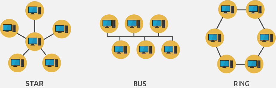
Deep Dives: - Topologies Fundamentals - Basic topology types (star, mesh, ring, bus) - Network Topologies - Physical vs logical topologies - Topologies Review - Advanced topology concepts

Design Process: - Network Design - Complete design methodology - Network Simulation - Testing topology designs - Optimization - Topology optimization

Routing: - Routing Fundamentals - Routing in different topologies - Routing Labs - Configure routing for topologies

Architecture: - WSN Architectures - Sensor network topologies - Hierarchical Design - Multi-tier topologies - Edge Computing - Distributed topology design

IoT Protocols: - Zigbee Architecture - Mesh topology protocol - Wi-Fi Mesh - Wi-Fi mesh topologies

Learning: - Simulations Hub - Topology visualization tools

780.2 Prerequisites

Before diving into this chapter, you should be familiar with:

• Network Topologies: Fundamentals: Understanding basic topology types (star, mesh, ring, bus) and the difference between physical and logical topologies is essential for creating professional network diagrams and documentation
• Networking Basics: Knowledge of network devices, cabling standards, and wireless protocols provides the foundation for planning physical installations and cable runs
• Layered Network Models: Understanding how protocols operate at different layers helps you design logical topologies that accurately represent data flow and network operation

780.3 🌱 Getting Started (For Beginners)

TipFor Beginners: Turning Concepts into Topology Diagrams

In the fundamentals chapter you learned the names and properties of star, mesh, ring, and bus topologies. This lab chapter is about drawing and documenting real networks using those ideas.

• If you have access to tools like draw.io, Packet Tracer, or Visio:
  • Recreate the example diagrams, then redraw your own home or lab network using the same symbols.
  • Focus on clearly labelling devices, links, and subnets rather than perfection.
• If you only have pen and paper:
  • Sketch logical diagrams first (who talks to whom), then add physical details (where devices sit on a floor plan).

Checklist for a beginner‑friendly topology diagram:

Item	Question to ask yourself
Devices	Did I include all gateways, switches, and APs?
Links	Are all links drawn and labelled (Ethernet, Wi-Fi)?
Addresses	Did I show subnets or VLANs where they matter?
Legend	Did I include a small legend explaining symbols?

If you feel rusty on the difference between physical and logical topologies, reread topologies-fundamentals.qmd first, then return here and treat the labs as a guided drawing exercise.

780.4 Drawing Network Topologies

⏱️ ~15 min | ⭐⭐ Intermediate | 📋 P07.C28.U01

Figure 780.1: Types of visual representation in network diagrams - logical vs physical layouts

780.4.1 Logical Topology Drawing

Tools: - Hand-drawn: Quick for informal design, brainstorming - CAD software: Professional, consistent, standardized - Microsoft Visio - Cisco Packet Tracer - draw.io (free, web-based) - Lucidchart

Example: ARPANET c.1970 (hand-drawn)

Original Internet topology was hand-drawn on paper:

• Nodes represented as circles
• Lines showed connections
• Simple but effective for early network

Figure 780.2: Sample physical topology with distance measurements

Figure 780.3: Sample physical topology on office floorplan

Figure 780.4: Sample physical topology design process

Figure 780.5: Wireless network coverage planning with Cisco WCS

Figure 780.6: Physical topology documentation example

Modern best practices: - Use consistent symbols - Label all devices and interfaces - Include IP addressing information - Show logical groupings (VLANs, subnets) - Indicate key protocols used

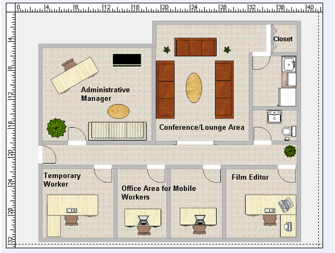
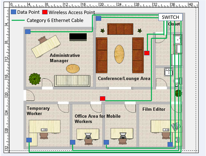
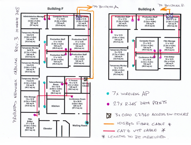
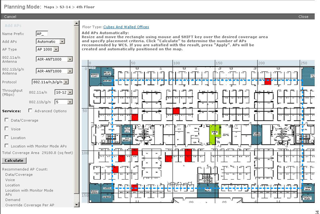
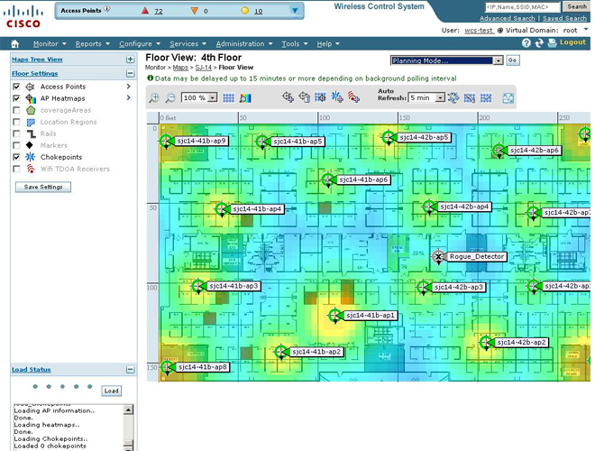
780.4.2 Physical Topology Drawing

Requirements: - Building floor plans or site maps - Device location information - Cable pathway constraints - Wireless propagation characteristics

Process: 1. Import floor plan (to scale) 2. Mark device locations 3. Plan cable routes (avoiding obstacles) 4. Calculate cable lengths 5. Show wireless coverage (for Wi-Fi/LoRa) 6. Document wall materials (for RF planning)

Specialized software: - Cisco Prime Infrastructure - Wireless planning - Ekahau - Wi-Fi site surveys and design - AutoCAD - Detailed construction plans - SketchUp - 3D visualization

---

780.5 IoT-Specific Topology Considerations

⏱️ ~12 min | ⭐⭐ Intermediate | 📋 P07.C28.U02

Figure 780.7: Hierarchical network design model showing access, distribution, and core layers

780.5.1 Unique IoT Challenges

1. Massive Device Count

Traditional network: 100-1000 devices IoT network: 10,000+ devices possible

Solution: - Multiple topology diagrams (by type) - Tabular device listings - Hierarchical grouping

2. Heterogeneous Devices

Different device types require different symbols:

%%{init: {'theme': 'base', 'themeVariables': { 'primaryColor': '#2C3E50', 'primaryTextColor': '#fff', 'primaryBorderColor': '#16A085', 'lineColor': '#16A085', 'secondaryColor': '#E67E22', 'tertiaryColor': '#ecf0f1'}}}%%
graph TB
    Gateway["IoT Gateway"]
    Sensor1["Temperature<br/>Sensor"]
    Sensor2["Motion<br/>Sensor"]
    Camera["IP Camera"]
    Actuator["Smart<br/>Thermostat"]
    Cloud["Cloud Platform"]

    Sensor1 & Sensor2 & Camera & Actuator -->|"Wi-Fi/Zigbee"| Gateway
    Gateway -->|"Internet"| Cloud

    style Gateway fill:#2C3E50,stroke:#16A085,stroke-width:3px,color:#fff
    style Sensor1 fill:#16A085,stroke:#2C3E50,stroke-width:2px,color:#fff
    style Sensor2 fill:#16A085,stroke:#2C3E50,stroke-width:2px,color:#fff
    style Camera fill:#E67E22,stroke:#2C3E50,stroke-width:2px
    style Actuator fill:#E67E22,stroke:#2C3E50,stroke-width:2px
    style Cloud fill:#7F8C8D,stroke:#2C3E50,stroke-width:2px

Figure 780.8: Smart Home Star Topology with Central Gateway

%%{init: {'theme': 'base', 'themeVariables': { 'primaryColor': '#2C3E50', 'primaryTextColor': '#fff', 'primaryBorderColor': '#16A085', 'lineColor': '#16A085', 'secondaryColor': '#E67E22', 'tertiaryColor': '#7F8C8D'}}}%%
graph TB
    subgraph STAR["Star Topology"]
        SG["Gateway<br/>SPOF"]
        S1["Sensor 1"]
        S2["Sensor 2"]
        S3["Sensor 3"]
        S1 --> SG
        S2 --> SG
        S3 --> SG
    end

    subgraph MESH["Mesh Topology"]
        M1["Node 1"]
        M2["Node 2"]
        M3["Node 3"]
        M4["Node 4"]
        M1 <--> M2
        M1 <--> M3
        M2 <--> M4
        M3 <--> M4
        M2 <--> M3
    end

    STAR -->|"Gateway fails<br/>ALL devices offline"| FAIL1["100% Outage"]
    MESH -->|"One node fails<br/>Traffic reroutes"| FAIL2["0% Outage<br/>(redundant paths)"]

    style SG fill:#E74C3C,stroke:#2C3E50,color:#fff
    style FAIL1 fill:#E74C3C,stroke:#2C3E50,color:#fff
    style FAIL2 fill:#16A085,stroke:#2C3E50,color:#fff
    style M1 fill:#16A085,stroke:#2C3E50,color:#fff
    style M2 fill:#16A085,stroke:#2C3E50,color:#fff
    style M3 fill:#16A085,stroke:#2C3E50,color:#fff
    style M4 fill:#16A085,stroke:#2C3E50,color:#fff

Figure 780.9: Alternative View: Topology Failure Analysis - While the device topology diagram shows the physical layout, this comparison highlights the critical difference in fault tolerance. Star topologies have a Single Point of Failure (SPOF) - if the gateway fails, 100% of devices go offline. Mesh topologies provide redundant paths - when one node fails, traffic automatically reroutes through alternate paths with zero outage. This trade-off between simplicity (star) and reliability (mesh) is fundamental to IoT network design decisions. {fig-alt=“Side-by-side comparison of Star vs Mesh topology failure modes. Star topology shows Gateway as Single Point of Failure (SPOF) in red, with three sensors connected. Gateway failure causes 100% outage. Mesh topology shows four interconnected nodes with multiple paths between them in teal. One node failure causes 0% outage due to redundant paths allowing traffic rerouting.”}

Recommendation: Create symbol legend for each topology

3. Multiple Network Types

IoT systems often use multiple protocols simultaneously:

%%{init: {'theme': 'base', 'themeVariables': { 'primaryColor': '#2C3E50', 'primaryTextColor': '#fff', 'primaryBorderColor': '#16A085', 'lineColor': '#16A085', 'secondaryColor': '#E67E22', 'tertiaryColor': '#ecf0f1'}}}%%
graph TB
    subgraph "Wi-Fi Network"
        Gateway["Gateway"]
        Camera["IP Camera"]
        Display["Display"]
    end

    subgraph "Zigbee Mesh"
        ZHub["Zigbee Hub"]
        Light1["Smart Light 1"]
        Light2["Smart Light 2"]
        Switch["Smart Switch"]
    end

    subgraph "BLE Network"
        Phone["Smartphone"]
        Watch["Smart Watch"]
        Band["Fitness Band"]
    end

    Camera & Display -->|"Wi-Fi"| Gateway
    Light1 & Light2 & Switch -.->|"Zigbee"| ZHub
    Watch & Band -.->|"BLE"| Phone
    ZHub --> Gateway
    Phone --> Gateway

    style Gateway fill:#2C3E50,stroke:#16A085,stroke-width:3px,color:#fff
    style ZHub fill:#16A085,stroke:#2C3E50,stroke-width:2px,color:#fff
    style Phone fill:#E67E22,stroke:#2C3E50,stroke-width:2px

Figure 780.10: Multi-Protocol Smart Home with Wi-Fi, Zigbee, and BLE Networks

Solution: Separate topologies by protocol, or use color coding

4. Wireless-Dominant

Many IoT devices are wireless: - Battery-powered sensors (no wires) - Mobile assets (vehicles, wearables) - Distributed outdoor sensors

Physical topology must show: - Gateway placement for coverage - Dead zones and interference - Redundant coverage areas

780.5.2 Example: Smart Building IoT Topology

Logical topology might separate:

1. HVAC sensors and actuators
   • Temperature sensors (Wi-Fi)
   • Humidity sensors (Wi-Fi)
   • Damper actuators (BACnet)
2. Security and access control
   • IP cameras (PoE Ethernet)
   • Door locks (Zigbee)
   • Motion sensors (Zigbee)
3. Lighting and energy
   • Smart lights (Zigbee mesh)
   • Power meters (Modbus TCP)
   • Solar inverters (proprietary)

Each system gets its own topology diagram for clarity.

---

780.6 Topology Selection for IoT

⏱️ ~10 min | ⭐⭐ Intermediate | 📋 P07.C28.U03

780.6.1 Decision Matrix

Topology	Best For	Avoid When
Star	Centralized control, small-medium networks	Need redundancy, gateway is bottleneck
Extended Star	Large buildings, campus networks	Simple deployments (overkill)
Bus	Short-distance, low-cost (I2C, CAN)	Need high reliability
Ring	Predictable performance, industrial	Need flexibility, easy reconfiguration
Full Mesh	Critical systems, maximum uptime	Cost-sensitive, many devices
Partial Mesh	Balance cost/redundancy	Very simple or very critical systems

780.6.2 IoT Application Examples

Smart Home: - Primary: Star topology (all sensors → hub) - Backup: Partial mesh (Zigbee for lighting) - Rationale: Central control, easy management

Industrial Monitoring: - Primary: Extended star (multiple PLCs → SCADA) - Secondary: Ring (fiber backbone for redundancy) - Rationale: Scalable, fault-tolerant

Smart Agriculture: - Primary: Star-of-stars (LoRaWAN sensors → gateway(s)) - Rationale: Wide area coverage with minimal relay complexity for battery-powered devices

Smart City: - Primary: Partial mesh (streetlight gateways) - Secondary: Star (sensors → gateway) - Rationale: Coverage vs cost balance

---

780.7 💻 Hands-On Lab: Network Topology Design

780.7.1 Lab: Draw an IoT Smart Home Topology

Objective: Create logical and physical topologies for a smart home.

Devices: - 1× Internet gateway/router - 1× Zigbee hub - 3× Wi-Fi cameras - 5× Zigbee smart lights - 4× Wi-Fi temperature sensors - 2× Wi-Fi smart plugs - 1× Smart TV (Wi-Fi)

Task 1: Logical Topology

Draw logical topology showing: - Device types (use symbols or icons) - Connectivity (Wi-Fi vs Zigbee) - IP network ranges - Data flow to cloud services

Recommended tool: draw.io or Cisco Packet Tracer

Task 2: Physical Topology

Draw physical layout on house floor plan: - Gateway location - Camera placement (coverage areas) - Zigbee hub central location - Wi-Fi coverage from router - Identify potential dead zones

Expected deliverables: 1. Logical topology diagram (PDF) 2. Physical topology on floor plan (PDF) 3. Brief explanation of topology choices

---

780.8 Knowledge Check

Test your understanding of network topology design, physical vs logical topologies, and mesh network scalability with these questions.

NoteAuto-Gradable Quick Check

Question: A network is wired in a physical star, but behaves like a logical bus. Is this possible?

💡 Explanation: B. With an Ethernet hub (shared medium), frames are repeated to all ports, so the LAN behaves like a bus even though it’s cabled as a star.

Question: A network with 8 devices uses a full mesh. How many direct connections exist?

💡 Explanation: C. Full mesh has n(n−1)/2 links, so 8×7/2 = 28.

Question: Which topology is best for battery-powered outdoor sensors spread across a large farm?

💡 Explanation: A. LPWAN deployments like LoRaWAN typically use a star-of-stars model; adding gateways extends coverage without requiring battery-powered nodes to relay traffic.

Question: What is the PRIMARY purpose of a physical topology diagram?

💡 Explanation: B. Physical topology focuses on the real-world layout used for installation planning, coverage, and physical-layer troubleshooting.

780.9 🎯 Quiz: Test Your Understanding

NoteQuestion 1: Physical vs Logical

A network has devices physically wired in a star configuration (all cables to a central hub, or a patch panel feeding a hub), but operates logically as a bus. Is this possible?

A) No, physical and logical topologies must match B) Yes, if the central device is a hub/shared medium (physical star, logical bus) C) Only if using wireless D) Only in IoT networks

Show Answer

Answer: B) Yes, if the central device is a hub/shared medium (physical star, logical bus)

Explanation: - Physical star: All devices connect to a central hub/switch via individual cables - Logical bus: If the central device is an Ethernet hub (shared medium), frames are repeated to all ports (CSMA/CD)

This is possible, but note that modern switched Ethernet is physically a star and logically closer to point-to-point links (no shared collisions in full-duplex).

Key principle: Physical and logical topologies can be different.

NoteQuestion 2: Mesh Topology

A Zigbee network with 8 devices uses full mesh topology. How many direct connections exist?

A) 8 B) 16 C) 28 D) 64

Show Answer

Answer: C) 28

Formula: For n devices in full mesh: n(n-1)/2 connections

Calculation: - n = 8 devices - Connections = 8 × 7 / 2 = 56 / 2 = 28 connections

Why divide by 2? Each connection is bidirectional (Device A to Device B is the same as Device B to Device A).

Practical implication: Full mesh becomes expensive very quickly! 10 devices = 45 connections, 20 devices = 190 connections.

NoteQuestion 3: IoT Topology Selection

Which topology is best for battery-powered outdoor sensors spread across a large farm?

A) Star (sensors → one or more gateways, e.g., LoRaWAN star-of-stars) B) Bus (shared cable) C) Ring (circular connections) D) Partial mesh (multi-hop routing between sensors)

Show Answer

Answer: A) Star (sensors → one or more gateways, e.g., LoRaWAN star-of-stars)

Reasoning: - Large area: Sensors spread far apart, may exceed single gateway range - Battery-powered: Need low-power protocol (e.g., LPWAN vs Wi-Fi) - Outdoor: No existing infrastructure (wired options not viable) - Star-of-stars: Gateways provide coverage; adding gateways is usually easier than requiring battery nodes to relay traffic

Why not others: - Bus/Ring: Not practical to deploy/maintain outdoors - Partial mesh: Relays add complexity and can drain the batteries of nodes that must forward traffic

Real-world example: Smart agriculture often uses LoRaWAN (star-of-stars): sensors uplink to one or more gateways, which forward data to the network server.

NoteQuestion 4: Topology Documentation

What is the PRIMARY purpose of a physical topology diagram?

A) Show how data flows through the network B) Show actual device locations and cable routes C) Show IP addressing scheme D) Show protocol configuration

Show Answer

Answer: B) Show actual device locations and cable routes

Physical topology is used for: - ✅ Installation planning (where to place devices) - ✅ Cable length calculations - ✅ Wireless coverage planning - ✅ Troubleshooting physical layer issues - ✅ Facility management

Logical topology is used for: - Network operation understanding (A) - IP addressing (C) - Protocol configuration (D)

Remember: Physical = actual layout, Logical = operation/flow

---

780.10 🐍 Python Implementations

780.10.1 Implementation 1: Network Topology Generator and Visualizer

Expected Output:

======================================================================
NETWORK TOPOLOGY GENERATOR
======================================================================

1. STAR TOPOLOGY (5 devices)
----------------------------------------------------------------------

Topology: star
Nodes: 6, Links: 5

Connections:
  Central ↔ Device1
  Central ↔ Device2
  Central ↔ Device3
  Central ↔ Device4
  Central ↔ Device5

Statistics:
  Connectivity ratio: 33.33%
  Avg connections/node: 1.7

2. RING TOPOLOGY (6 nodes)
----------------------------------------------------------------------

Topology: ring
Nodes: 6, Links: 6

Connections:
  Node1 ↔ Node2
  Node2 ↔ Node3
  Node3 ↔ Node4
  Node4 ↔ Node5
  Node5 ↔ Node6
  Node6 ↔ Node1

Statistics:
  Connectivity ratio: 40.00%

3. FULL MESH TOPOLOGY (5 nodes)
----------------------------------------------------------------------

Topology: full_mesh
Nodes: 5, Links: 10

Connections:
  Node1 ↔ Node2
  Node1 ↔ Node3
  Node1 ↔ Node4
  Node1 ↔ Node5
  Node2 ↔ Node3
  Node2 ↔ Node4
  Node2 ↔ Node5
  Node3 ↔ Node4
  Node3 ↔ Node5
  Node4 ↔ Node5

Statistics:
  Total links: 10 (Formula: n(n-1)/2 = 5×4/2 = 10)
  Connectivity ratio: 100.00% (100% = full mesh)

4. PARTIAL MESH TOPOLOGY (8 nodes, 40% connection probability)
----------------------------------------------------------------------

Topology: partial_mesh
Nodes: 8, Links: 12

Connections:
  [12 random connections displayed...]

Statistics:
  Total links: 12 out of 28 possible
  Connectivity ratio: 42.86%

Key Concepts: - Star: Single point of failure (central node), easy to manage - Ring: Equal access, predictable performance, one break affects all - Mesh: Full mesh = n(n-1)/2 connections, expensive but highly redundant - Partial Mesh: Balance between cost and redundancy

---

780.10.2 Implementation 2: Topology Analyzer (Network Metrics)

Expected Output:

======================================================================
TOPOLOGY ANALYZER
======================================================================

1. STAR TOPOLOGY ANALYSIS
----------------------------------------------------------------------
Path D1 → D4:
  Shortest: D1 → Central → D4
  Hops: 2
  Total paths found: 1
  Redundant paths: 0

Network Metrics:
  Diameter: 2 hops
  Average path length: 1.67 hops
  Single points of failure: ['Central']
  Resilience score: 0.27 (0-1 scale)


2. PARTIAL MESH TOPOLOGY ANALYSIS
----------------------------------------------------------------------
Path N1 → N5:
  Shortest: N1 → N3 → N5
  Hops: 2
  All paths:
    Path 1: N1 → N3 → N5
    Path 2: N1 → N3 → N4 → N5
    Path 3: N1 → N2 → N3 → N5
    Path 4: N1 → N2 → N4 → N5

Network Metrics:
  Diameter: 2 hops
  Average path length: 1.80 hops
  Single points of failure: None
  Resilience score: 0.74 (0-1 scale)


3. TOPOLOGY COMPARISON
----------------------------------------------------------------------
Metric                    Star            Partial Mesh
----------------------------------------------------------------------
Diameter                  2 hops          2 hops
SPOFs                     Yes (Central)   None
Resilience                Low             Higher

---

780.10.3 Implementation 3: Mesh Network Scalability Calculator

Expected Output:

MESH NETWORK SCALABILITY ANALYSIS
==========================================================================================
Cost per link: $100.00
Partial mesh ratio: 30%
==========================================================================================
Nodes    Full Mesh       Partial Mesh    Full Cost       Partial Cost    Savings
         Links           Links           (USD)           (USD)           (%)
------------------------------------------------------------------------------------------
5        10              3               $10,000.00      $3,000.00       70.0%
10       45              13              $4,500.00       $1,350.00       70.0%
20       190             57              $19,000.00      $5,700.00       70.0%
50       1,225           367             $122,500.00     $36,750.00      70.0%
100      4,950           1,485           $495,000.00     $148,500.00     70.0%


DETAILED ANALYSIS: 20-node network
==========================================================================================
Nodes: 20

Full Mesh:
  Connections: 190
  Total cost: $19,000.00

Partial Mesh (30% connectivity):
  Connections: 57
  Total cost: $5,700.00
  Cost savings: $13,300.00 (70.0%)
  Estimated avg path length: 2.09 hops


BUDGET OPTIMIZATION
==========================================================================================
Budget $1,000 → Max 5 nodes (30% partial mesh)
Budget $5,000 → Max 19 nodes (30% partial mesh)
Budget $10,000 → Max 27 nodes (30% partial mesh)
Budget $50,000 → Max 62 nodes (30% partial mesh)


TOPOLOGY RECOMMENDATIONS
==========================================================================================

Small IoT sensor network, redundancy required:
  Nodes: 5
  Redundancy: True
  → Recommendation: Full mesh (only 10 links, affordable)

Small IoT sensor network, no redundancy required:
  Nodes: 5
  Redundancy: False
  → Recommendation: Star topology (simple, cost-effective)

Medium industrial network, redundancy required:
  Nodes: 15
  Redundancy: True
  → Recommendation: Partial mesh with 40-60% connectivity

Large smart building, redundancy required:
  Nodes: 50
  Redundancy: True
  → Recommendation: Partial mesh with 20-30% connectivity (1225 full mesh links would be excessive)

Key Insights: - Full mesh connections grow quadratically: n(n-1)/2 - 100 nodes = 4,950 connections (impractical!) - Partial mesh reduces cost dramatically (70% savings at 30% connectivity) - Star topology best for small, cost-sensitive deployments - Partial mesh best for medium-large networks needing redundancy

---

780.11 💻 Advanced Hands-On Labs

780.11.1 Lab 3: ESP32 Network Topology Discovery Simulator

Objective: Simulate network topology discovery on ESP32.

Hardware Required: - ESP32 development board - USB cable - Computer with Arduino IDE

Code:

#include <Wi-Fi.h>
#include <vector>
#include <map>

// Network node structure
struct Node {
  String id;
  std::vector<String> neighbors;
  bool discovered;
  int hopCount;
};

// Simulated network topology
std::map<String, Node> network;

void setup() {
  Serial.begin(115200);
  delay(2000);

  Serial.println("\n╔════════════════════════════════════════╗");
  Serial.println("║  Network Topology Discovery Simulator ║");
  Serial.println("║  ESP32 BFS-based Discovery             ║");
  Serial.println("╚════════════════════════════════════════╝\n");

  // Create sample topology (partial mesh)
  createSampleTopology();

  // Display topology
  displayTopology();

  // Run topology discovery
  Serial.println("\n═══════════════════════════════════════════════════");
  Serial.println("Running Topology Discovery (BFS from N1)");
  Serial.println("═══════════════════════════════════════════════════\n");

  discoverTopology("N1");

  // Analyze topology
  analyzeTopology();
}

void loop() {
  // Discovery runs once in setup()
}

void createSampleTopology() {
  // Create nodes
  network["N1"] = {"N1", {"N2", "N3"}, false, 0};
  network["N2"] = {"N2", {"N1", "N3", "N4"}, false, 0};
  network["N3"] = {"N3", {"N1", "N2", "N5"}, false, 0};
  network["N4"] = {"N4", {"N2", "N5"}, false, 0};
  network["N5"] = {"N5", {"N3", "N4"}, false, 0};

  Serial.println("Sample Topology Created (Partial Mesh):");
  Serial.println("  N1 connects to: N2, N3");
  Serial.println("  N2 connects to: N1, N3, N4");
  Serial.println("  N3 connects to: N1, N2, N5");
  Serial.println("  N4 connects to: N2, N5");
  Serial.println("  N5 connects to: N3, N4");
}

void displayTopology() {
  Serial.println("\n┌─────────────────────────────────────────┐");
  Serial.println("│          Network Topology               │");
  Serial.println("└─────────────────────────────────────────┘");
  Serial.println("Node  Neighbors            Degree");
  Serial.println("────────────────────────────────────────────");

  for (auto& pair : network) {
    Node& node = pair.second;
    String neighbors = "";
    for (size_t i = 0; i < node.neighbors.size(); i++) {
      neighbors += node.neighbors[i];
      if (i < node.neighbors.size() - 1) neighbors += ", ";
    }

    char line[60];
    sprintf(line, "%-5s %-20s %d", node.id.c_str(), neighbors.c_str(),
            node.neighbors.size());
    Serial.println(line);
  }
  Serial.println("────────────────────────────────────────────");
}

void discoverTopology(String startNode) {
  // BFS-based topology discovery
  std::vector<String> queue;
  queue.push_back(startNode);

  network[startNode].discovered = true;
  network[startNode].hopCount = 0;

  int round = 0;

  while (!queue.empty()) {
    Serial.printf("\n--- Discovery Round %d ---\n", round++);

    std::vector<String> nextQueue;

    for (const String& currentId : queue) {
      Node& current = network[currentId];

      Serial.printf("Exploring %s (hop %d):\n", currentId.c_str(),
                    current.hopCount);

      // Discover neighbors
      for (const String& neighborId : current.neighbors) {
        if (!network[neighborId].discovered) {
          network[neighborId].discovered = true;
          network[neighborId].hopCount = current.hopCount + 1;
          nextQueue.push_back(neighborId);

          Serial.printf("  → Discovered %s at hop %d\n",
                       neighborId.c_str(), network[neighborId].hopCount);
        } else {
          Serial.printf("  → %s already discovered\n", neighborId.c_str());
        }
      }
    }

    queue = nextQueue;
  }

  Serial.println("\n✓ Topology discovery complete!");
}

void analyzeTopology() {
  Serial.println("\n\n╔════════════════════════════════════════╗");
  Serial.println("║         Topology Analysis              ║");
  Serial.println("╚════════════════════════════════════════╝");

  // Calculate statistics
  int totalNodes = network.size();
  int totalLinks = 0;
  int maxDegree = 0;
  int minDegree = 999;
  int diameter = 0;

  for (auto& pair : network) {
    Node& node = pair.second;
    int degree = node.neighbors.size();

    totalLinks += degree;
    maxDegree = max(maxDegree, degree);
    minDegree = min(minDegree, degree);
    diameter = max(diameter, node.hopCount);
  }

  totalLinks /= 2;  // Each link counted twice

  // Calculate maximum possible links (full mesh)
  int maxPossibleLinks = totalNodes * (totalNodes - 1) / 2;
  float connectivity = (float)totalLinks / maxPossibleLinks * 100.0;

  float avgDegree = (float)(totalLinks * 2) / totalNodes;

  // Display statistics
  Serial.printf("\nNodes: %d\n", totalNodes);
  Serial.printf("Links: %d\n", totalLinks);
  Serial.printf("Max possible links (full mesh): %d\n", maxPossibleLinks);
  Serial.printf("Connectivity ratio: %.1f%%\n", connectivity);
  Serial.printf("\nDegree statistics:\n");
  Serial.printf("  Min degree: %d\n", minDegree);
  Serial.printf("  Max degree: %d\n", maxDegree);
  Serial.printf("  Avg degree: %.2f\n", avgDegree);
  Serial.printf("\nNetwork diameter: %d hops\n", diameter);

  // Topology type classification
  Serial.println("\nTopology classification:");
  if (totalLinks == totalNodes - 1) {
    Serial.println("  → Tree topology (minimal connectivity)");
  } else if (connectivity >= 95) {
    Serial.println("  → Full mesh (maximum redundancy)");
  } else if (connectivity >= 40) {
    Serial.println("  → Partial mesh (good redundancy)");
  } else if (maxDegree == totalNodes - 1 && minDegree == 1) {
    Serial.println("  → Star topology (central hub)");
  } else {
    Serial.println("  → Hybrid topology");
  }

  // Recommendations
  Serial.println("\nRecommendations:");
  if (connectivity < 30) {
    Serial.println("  ⚠ Low connectivity - consider adding links for redundancy");
  }
  if (diameter > 3) {
    Serial.println("  ⚠ High diameter - long paths may cause latency");
  }
  if (maxDegree > totalNodes / 2) {
    Serial.println("  ⚠ High-degree node detected - potential bottleneck");
  }
  if (connectivity >= 50) {
    Serial.println("  ✓ Good redundancy level");
  }
  if (diameter <= 2) {
    Serial.println("  ✓ Low diameter - efficient routing");
  }

  Serial.println("\n═══════════════════════════════════════════════════");
  Serial.println("Analysis Complete");
  Serial.println("═══════════════════════════════════════════════════\n");
}

Tip🎮 Try It: ESP32 Network Simulator

Run this topology discovery algorithm in the browser! The simulation demonstrates BFS-based network discovery, calculating connectivity metrics, network diameter, and topology classification.

What to Observe:

• BFS Discovery: Watch how the algorithm explores nodes level by level
• Hop Counts: Each node gets assigned a distance from the start node
• Topology Metrics: Connectivity ratio, degree distribution, diameter
• Try: Modify the createSampleTopology() function to create different network structures (star, ring, full mesh)

Expected Serial Output:

╔════════════════════════════════════════╗
║  Network Topology Discovery Simulator ║
║  ESP32 BFS-based Discovery             ║
╚════════════════════════════════════════╝

Sample Topology Created (Partial Mesh):
  N1 connects to: N2, N3
  N2 connects to: N1, N3, N4
  N3 connects to: N1, N2, N5
  N4 connects to: N2, N5
  N5 connects to: N3, N4

┌─────────────────────────────────────────┐
│          Network Topology               │
└─────────────────────────────────────────┘
Node  Neighbors            Degree
────────────────────────────────────────────
N1    N2, N3               2
N2    N1, N3, N4           3
N3    N1, N2, N5           3
N4    N2, N5               2
N5    N3, N4               2
────────────────────────────────────────────

═══════════════════════════════════════════════════
Running Topology Discovery (BFS from N1)
═══════════════════════════════════════════════════


--- Discovery Round 0 ---
Exploring N1 (hop 0):
  → Discovered N2 at hop 1
  → Discovered N3 at hop 1

--- Discovery Round 1 ---
Exploring N2 (hop 1):
  → N1 already discovered
  → N3 already discovered
  → Discovered N4 at hop 2
Exploring N3 (hop 1):
  → N1 already discovered
  → N2 already discovered
  → Discovered N5 at hop 2

--- Discovery Round 2 ---
Exploring N4 (hop 2):
  → N2 already discovered
  → N5 already discovered
Exploring N5 (hop 2):
  → N3 already discovered
  → N4 already discovered

✓ Topology discovery complete!


╔════════════════════════════════════════╗
║         Topology Analysis              ║
╚════════════════════════════════════════╝

Nodes: 5
Links: 6
Max possible links (full mesh): 10
Connectivity ratio: 60.0%

Degree statistics:
  Min degree: 2
  Max degree: 3
  Avg degree: 2.40

Network diameter: 2 hops

Topology classification:
  → Partial mesh (good redundancy)

Recommendations:
  ✓ Good redundancy level
  ✓ Low diameter - efficient routing

═══════════════════════════════════════════════════
Analysis Complete
═══════════════════════════════════════════════════

---

780.11.2 Lab 4: Python Interactive Topology Visualizer

Objective: Create interactive network topology visualizations with NetworkX and Matplotlib.

Setup:

pip install networkx matplotlib

Code:

This creates a comprehensive visualization showing: 1. Star topology with central hub highlighted 2. Ring topology with directional flow 3. Bus topology with shared medium 4. Full mesh with all connections 5. Partial mesh with selective connections 6. Tree topology with hierarchical structure

Each subplot includes statistics about nodes, links, and key characteristics.

---

780.12 Summary

• Topology documentation requires both logical diagrams (communication flow) and physical diagrams (device placement and cable runs)
• Professional tools like Visio, Cisco Packet Tracer, draw.io, and Ekahau enable standardized topology design and wireless planning
• IoT-specific challenges include massive device counts, heterogeneous protocols, and wireless-dominant deployments requiring specialized visualization
• Topology selection depends on fault tolerance needs, scalability requirements, and cost constraints for specific IoT applications
• Mesh network scalability follows n(n-1)/2 formula - partial mesh balances cost and redundancy better than full mesh for large deployments
• Topology analysis uses graph theory metrics like diameter, average path length, single points of failure, and resilience scores
• Python implementations enable automated topology generation, network analysis, path finding, and scalability calculations for IoT design

780.13 Visual Reference Gallery

Explore these AI-generated visualizations that support topology design concepts.

NoteVisual: Mesh Network Formation

Mesh Network Formation

Understanding how mesh networks form dynamically helps in designing self-configuring IoT deployments.

NoteVisual: Mesh Network Architecture

Mesh Network

Mesh networks provide resilience through path redundancy, making them ideal for critical IoT applications.

NoteVisual: Ring Topology for IoT

Ring Topology IoT

Ring topologies suit industrial IoT applications where deterministic timing and controlled access are required.

NoteVisual: Bluetooth Mesh Topology

Bluetooth Mesh Topology

Bluetooth Mesh provides a standardized approach to building IoT mesh networks with commercial off-the-shelf devices.

780.14 What’s Next

With topology design skills mastered, continue to:

• Network Topologies: Comprehensive Review: Advanced topology concepts, quiz questions, and knowledge checks
• Transport Protocols: Fundamentals: TCP and UDP characteristics for IoT communication
• Routing Fundamentals: How data flows through topologies using routing protocols
• 6LoWPAN Architecture: IPv6 adaptation layer for constrained IoT networks