708  RPL Introduction and Core Concepts

NoteLearning Objectives

By the end of this section, you will be able to:

• Understand why traditional routing protocols don’t work for Low-Power and Lossy Networks (LLNs)
• Explain RPL as a distance-vector routing protocol for IoT
• Understand DODAG (Destination Oriented Directed Acyclic Graph) topology
• Explain the RANK concept and loop prevention mechanisms

708.1 Prerequisites

Before diving into this chapter, you should be familiar with:

• Routing Fundamentals: Knowledge of basic routing concepts, routing tables, and distance-vector protocols helps you understand RPL’s routing decisions
• 6LoWPAN Fundamentals: RPL typically operates with 6LoWPAN, so familiarity with IPv6 header compression and adaptation layer mechanisms is important
• Wireless Sensor Networks: Understanding WSN energy constraints and multi-hop communication patterns explains RPL’s design choices and optimization strategies

NoteRelated Chapters

This Series: - RPL Introduction - This chapter - RPL DODAG Construction and Modes - Building DODAGs and routing modes - RPL Traffic Patterns and Design - Traffic patterns and network design lab - RPL Production and Summary - Production framework and key takeaways

Comparisons: - Routing Fundamentals - Distance-vector vs link-state routing - 6LoWPAN Fundamentals - RPL integration with IPv6 compression - Thread Comprehensive Review - Alternative routing in Thread/Matter networks

Hands-On: - RPL Production and Review - Storing vs Non-Storing mode deployment - Simulations Hub - Test RPL DODAG formation in simulators

TipFor Beginners: What is RPL?

Imagine a smart building with 500 sensors spread across 20 floors. Sensor data needs to reach a central controller on the ground floor, but not every sensor can communicate directly—wireless signals don’t penetrate all walls and floors. Sensors need to relay messages through other sensors to reach the destination. This is called multi-hop routing.

But here’s the problem: traditional Internet routing protocols (like those used in Wi-Fi routers) assume devices have plenty of battery power, memory, and processing capability. IoT sensors have tiny batteries, minimal memory, and weak processors. Running traditional routing protocols would drain batteries in days.

RPL (Routing Protocol for Low-power and Lossy networks) is designed specifically for this challenge. It creates a tree-like structure where all data flows “upward” toward a central point (called the “root”), like water flowing downhill to a river. This structure is called a DODAG (Destination-Oriented Directed Acyclic Graph)—a fancy way of saying “tree where all paths lead to the root without loops.”

Think of it like an organization chart: employees report to managers, managers report to directors, directors report to the CEO. Messages flow up the hierarchy efficiently without getting stuck in circles. RPL does this for sensors, ensuring data reaches the gateway while conserving precious battery power.

Term	Simple Explanation
RPL	Routing Protocol for Low-power and Lossy networks—designed for IoT
Multi-hop	Messages relay through multiple devices to reach destination
DODAG	Tree structure where all paths lead to root (like org chart)
Root	Central node where all data ultimately flows (gateway/coordinator)
RANK	Device’s distance from root—like floors in a building
Upward Route	Data flowing from sensors toward root
Downward Route	Commands flowing from root toward specific sensors
LLN	Low-power and Lossy Network—constrained IoT environment

---

708.2 Introduction to RPL

⏱️ ~10 min | ⭐⭐ Intermediate | 📋 P07.C25.U01

RPL (IPv6 Routing Protocol for Low-Power and Lossy Networks) is a distance-vector routing protocol specifically designed for resource-constrained IoT devices operating in challenging network conditions.

IoT routers, like other devices in an IoT environment, are resource constrained. As they operate in Low Power and Lossy Networks (LLN), there are limitations that make it almost impossible to use traditional routing protocols.

%%{init: {'theme': 'base', 'themeVariables': { 'primaryColor': '#2C3E50', 'primaryTextColor': '#fff', 'primaryBorderColor': '#16A085', 'lineColor': '#16A085', 'secondaryColor': '#E67E22', 'tertiaryColor': '#7F8C8D'}}}%%
graph TB
    subgraph LLN["Low-Power and Lossy Network (LLN)"]
        L1["10-40% Packet Loss"]
        L2["Variable Link Quality"]
        L3["Asymmetric Links"]
        L4["Battery-Powered Devices"]
    end

    subgraph Constraints["IoT Device Constraints"]
        C1["CPU: 8-32 MHz"]
        C2["RAM: 10-128 KB"]
        C3["Flash: 32-512 KB"]
        C4["Power: Milliwatts"]
    end

    RPL["RPL Protocol<br/>Designed for LLNs"]

    LLN --> RPL
    Constraints --> RPL

    style LLN fill:#E67E22,stroke:#2C3E50,color:#fff
    style Constraints fill:#E67E22,stroke:#2C3E50,color:#fff
    style RPL fill:#2C3E50,stroke:#16A085,color:#fff,stroke-width:3px
    style L1 fill:#F8F9FA,stroke:#E67E22,color:#2C3E50
    style L2 fill:#F8F9FA,stroke:#E67E22,color:#2C3E50
    style L3 fill:#F8F9FA,stroke:#E67E22,color:#2C3E50
    style L4 fill:#F8F9FA,stroke:#E67E22,color:#2C3E50
    style C1 fill:#F8F9FA,stroke:#E67E22,color:#2C3E50
    style C2 fill:#F8F9FA,stroke:#E67E22,color:#2C3E50
    style C3 fill:#F8F9FA,stroke:#E67E22,color:#2C3E50
    style C4 fill:#F8F9FA,stroke:#E67E22,color:#2C3E50

Figure 708.1: LLN characteristics and IoT device constraints that drive RPL protocol design

{fig-alt=“Diagram showing Low-Power and Lossy Network characteristics (packet loss, variable links, asymmetric links, battery power) and IoT device constraints (limited CPU, RAM, flash, power) both pointing to RPL protocol as the designed solution”}

ImportantKnowledge Check

Test your understanding of these networking concepts.

NoteQuiz 1: Introduction to RPL

Question 9: In Storing mode RPL, when does a node send a DAO (Destination Advertisement Object) message?

Explanation: DAO messages build downward routes in RPL. A node sends DAO to its parent(s) to advertise: “I can reach these destinations.” This includes the node’s own address and any destinations learned from its children’s DAO messages. Example: Node E sends DAO to parent D saying “I can reach E.” Node D stores this in its routing table, then sends DAO to its parent C saying “I can reach D and E.” This propagates up to the root, building complete downward routing paths. DAO triggers: joining network, parent change, receiving DAO from child, periodic refresh. In Non-Storing mode, DAOs go directly to the root, not to parents. The root sends DAO-ACK to confirm receipt. This is distinct from DIO (advertise DODAG info) and DIS (request DODAG info).

708.3 RPL Specification

• Standard: RFC 6550 (IETF, March 2012)
• Type: Distance-vector routing protocol
• Network Layer: IPv6 (works with 6LoWPAN)
• Topology: DODAG (Destination Oriented Directed Acyclic Graph)
• Metrics: Flexible (hops, ETX, latency, energy, etc.)
• Use Case: Low-power, lossy networks with many-to-one traffic patterns

708.4 Why Not Use Existing Routing Protocols?

Traditional routing protocols like OSPF, RIP, and AODV were designed for different network characteristics. They don’t work well for IoT because:

708.4.1 Processing, Memory, and Power Constraints

%%{init: {'theme': 'base', 'themeVariables': { 'primaryColor': '#2C3E50', 'primaryTextColor': '#fff', 'primaryBorderColor': '#16A085', 'lineColor': '#16A085', 'secondaryColor': '#E67E22', 'tertiaryColor': '#7F8C8D'}}}%%
graph LR
    subgraph Traditional["Traditional Router<br/>(OSPF/RIP)"]
        T1["CPU: GHz multi-core"]
        T2["RAM: GB"]
        T3["Power: Watts"]
        T4["Complex routing tables"]
    end

    subgraph IoT["IoT Sensor"]
        I1["CPU: 32 MHz single"]
        I2["RAM: 32 KB"]
        I3["Power: mW battery"]
        I4["Parent pointer only"]
    end

    VS["Incompatible"]

    Traditional -.-> VS
    IoT -.-> VS

    style Traditional fill:#7F8C8D,stroke:#2C3E50,color:#fff
    style IoT fill:#16A085,stroke:#2C3E50,color:#fff
    style VS fill:#E67E22,stroke:#2C3E50,color:#fff,stroke-width:3px
    style T1 fill:#F8F9FA,stroke:#7F8C8D,color:#2C3E50
    style T2 fill:#F8F9FA,stroke:#7F8C8D,color:#2C3E50
    style T3 fill:#F8F9FA,stroke:#7F8C8D,color:#2C3E50
    style T4 fill:#F8F9FA,stroke:#7F8C8D,color:#2C3E50
    style I1 fill:#F8F9FA,stroke:#16A085,color:#2C3E50
    style I2 fill:#F8F9FA,stroke:#16A085,color:#2C3E50
    style I3 fill:#F8F9FA,stroke:#16A085,color:#2C3E50
    style I4 fill:#F8F9FA,stroke:#16A085,color:#2C3E50

Figure 708.2: Traditional router vs IoT sensor resource comparison showing incompatibility for standard protocols

{fig-alt=“Comparison showing traditional router requirements (GHz CPU, GB RAM, watts power, complex tables) versus IoT sensor constraints (32 MHz CPU, 32 KB RAM, milliwatts battery, parent pointer only) highlighting incompatibility”}

Traditional Protocols Require: - Complex routing tables: OSPF maintains link-state database of entire network - Frequent updates: RIP sends entire routing table every 30 seconds - Heavy processing: Link-state algorithms (Dijkstra’s shortest path) - Power-hungry: Constant listening and periodic broadcasts

IoT Constraints: - Microcontroller: 8-32 MHz, single core - RAM: 10-128 KB (vs GB in traditional routers) - Flash: 32-512 KB (limited code and data storage) - Power: Milliwatts (battery-powered, years of operation)

708.4.2 Single Metric Not Always Appropriate

Traditional protocols use single metric: - RIP: Hop count only - OSPF: Cost (usually based on bandwidth)

IoT requires multiple, context-dependent metrics: - Latency: Real-time monitoring (industrial sensors) - Reliability: Critical data (medical devices) - Energy: Battery-powered devices (maximize lifetime) - Bandwidth: Mixed traffic (sensors + actuators)

RPL Solution: Supports objective functions with multiple metrics

708.4.3 Multiple Routing Instances

IoT Scenario: Single physical network, multiple applications

%%{init: {'theme': 'base', 'themeVariables': { 'primaryColor': '#2C3E50', 'primaryTextColor': '#fff', 'primaryBorderColor': '#16A085', 'lineColor': '#16A085', 'secondaryColor': '#E67E22', 'tertiaryColor': '#7F8C8D'}}}%%
graph TB
    Physical["Same Physical Network<br/>100 IoT Devices"]

    subgraph Instance1["RPL Instance 1<br/>Latency Optimized"]
        I1_App["Temperature Monitoring"]
        I1_Metric["Metric: Minimize Latency"]
        I1_Parent["Fast parent selection"]
    end

    subgraph Instance2["RPL Instance 2<br/>Energy Optimized"]
        I2_App["Firmware Updates"]
        I2_Metric["Metric: Minimize Energy"]
        I2_Parent["Low-power parent selection"]
    end

    Physical --> Instance1
    Physical --> Instance2

    style Physical fill:#2C3E50,stroke:#16A085,color:#fff,stroke-width:3px
    style Instance1 fill:#16A085,stroke:#2C3E50,color:#fff
    style Instance2 fill:#E67E22,stroke:#2C3E50,color:#fff
    style I1_App fill:#F8F9FA,stroke:#16A085,color:#2C3E50
    style I1_Metric fill:#F8F9FA,stroke:#16A085,color:#2C3E50
    style I1_Parent fill:#F8F9FA,stroke:#16A085,color:#2C3E50
    style I2_App fill:#F8F9FA,stroke:#E67E22,color:#2C3E50
    style I2_Metric fill:#F8F9FA,stroke:#E67E22,color:#2C3E50
    style I2_Parent fill:#F8F9FA,stroke:#E67E22,color:#2C3E50

Figure 708.3: Multiple RPL instances on same network with different optimization objectives (latency vs energy)

{fig-alt=“Multiple RPL instances on same physical network: Instance 1 optimizes for latency (temperature monitoring) with fast parent selection, Instance 2 optimizes for energy (firmware updates) with low-power parent selection”}

Example: - Instance 1: Temperature monitoring (minimize latency) - Instance 2: Firmware updates (minimize energy, can be slower) - Same devices, different routing decisions based on application

708.4.4 Point-to-Multipoint Traffic Patterns

Traditional networks: Assume peer-to-peer traffic

IoT networks: Predominantly many-to-one traffic - Many sensors -> One gateway (cloud) - Data aggregation at root

RPL Optimization: Optimized for convergent traffic towards root

708.4.5 Lossy Links

Traditional networks: Assume reliable links (wired, enterprise Wi-Fi)

Low-Power and Lossy Networks (LLN): - High packet loss: 10-40% (vs < 1% wired) - Variable link quality: Interference, fading, obstacles - Asymmetric links: A can hear B, but B can’t hear A - Time-varying: Link quality changes over time

RPL Features for Lossy Networks: - Trickle timer: Adaptive control message frequency - ETX metric: Expected Transmission Count (accounts for retransmissions) - Loop avoidance: RANK prevents routing loops

NoteQuiz 2: Why Not Use Existing Routing Protocols?

Question 5: Why does RPL use the DODAG (Destination Oriented Directed Acyclic Graph) topology instead of allowing routing cycles?

Explanation: The DODAG (Directed Acyclic Graph) structure is fundamental to RPL’s loop prevention. By enforcing that RANK strictly increases along any path toward the root, cycles become impossible - a packet can never return to a node it has already visited. This is critical for resource-constrained IoT devices that can’t afford complex loop detection like spanning tree protocols. Traditional distance-vector protocols (RIP) can suffer from “count-to-infinity” problems during convergence. RPL’s RANK mechanism bounds this: if a node’s parent fails, it selects another parent with lower RANK, or increases its own RANK. The DAG structure is single-rooted per instance (though multiple instances can exist).

Question 11: Why is RPL classified as a “distance-vector” routing protocol rather than “link-state”?

Explanation: Distance-vector vs Link-state are fundamental routing paradigms:

Distance-Vector (RPL, RIP): - Node knows: “To reach root, forward to Parent X (next hop), cost is Y (distance/metric)” - Doesn’t know complete network topology - Routing info learned from neighbors’ advertisements - Lower memory, simpler computation - Example: Node E knows “Root is 4 hops via Parent D” but doesn’t know the full path or alternative routes

Link-State (OSPF, IS-IS): - Node knows complete network map: all nodes, all links, all costs - Computes best path using Dijkstra’s algorithm - Higher memory (store entire topology) - Faster convergence but more overhead

RPL uses distance-vector because IoT devices can’t afford to store and compute on complete network topology. The RANK value represents “distance” (in metric space) to root. “Vector” refers to the direction (next hop/parent).

708.5 RPL Core Concepts

708.5.1 Directed Acyclic Graph (DAG)

DAG = Directed Acyclic Graph

%%{init: {'theme': 'base', 'themeVariables': { 'primaryColor': '#2C3E50', 'primaryTextColor': '#fff', 'primaryBorderColor': '#16A085', 'lineColor': '#16A085', 'secondaryColor': '#E67E22', 'tertiaryColor': '#7F8C8D'}}}%%
graph TB
    A["Node A"]
    B["Node B"]
    C["Node C"]
    D["Node D"]
    E["Node E"]

    A --> B
    A --> C
    B --> D
    C --> D
    D --> E

    style A fill:#2C3E50,stroke:#16A085,color:#fff
    style B fill:#16A085,stroke:#2C3E50,color:#fff
    style C fill:#16A085,stroke:#2C3E50,color:#fff
    style D fill:#E67E22,stroke:#2C3E50,color:#fff
    style E fill:#7F8C8D,stroke:#2C3E50,color:#fff

Figure 708.4: Directed Acyclic Graph (DAG) with nodes connected by directed edges without cycles

{fig-alt=“Directed Acyclic Graph (DAG) example showing nodes A through E connected with directed arrows flowing downward, demonstrating no cycles - cannot return to same node following edges”}

Key Properties: - Directed: Edges have direction (arrows) - Acyclic: No cycles (cannot return to same node following edges) - Graph: Nodes connected by edges

Why DAG? - Loop-free routing: By definition, no cycles = no routing loops - Hierarchical structure: Natural parent-child relationships - Efficient aggregation: Data flows towards root(s)

708.5.2 DODAG (Destination Oriented DAG)

RPL uses DODAG: DAG with single root (destination)

%%{init: {'theme': 'base', 'themeVariables': { 'primaryColor': '#2C3E50', 'primaryTextColor': '#fff', 'primaryBorderColor': '#16A085', 'lineColor': '#16A085', 'secondaryColor': '#E67E22', 'tertiaryColor': '#7F8C8D'}}}%%
graph TB
    ROOT["ROOT<br/>(Single Destination)<br/>Rank: 0"]
    A["Node A<br/>Rank: 256"]
    B["Node B<br/>Rank: 256"]
    C["Node C<br/>Rank: 512"]
    D["Node D<br/>Rank: 512"]
    E["Node E<br/>Rank: 768"]
    F["Node F<br/>Rank: 768"]

    ROOT --> A
    ROOT --> B
    A --> C
    A --> D
    B --> D
    C --> E
    D --> F

    style ROOT fill:#2C3E50,stroke:#16A085,color:#fff,stroke-width:4px
    style A fill:#16A085,stroke:#2C3E50,color:#fff
    style B fill:#16A085,stroke:#2C3E50,color:#fff
    style C fill:#E67E22,stroke:#2C3E50,color:#fff
    style D fill:#E67E22,stroke:#2C3E50,color:#fff
    style E fill:#7F8C8D,stroke:#2C3E50,color:#fff
    style F fill:#7F8C8D,stroke:#2C3E50,color:#fff

Figure 708.5: DODAG topology with single ROOT (Rank 0) and hierarchical node ranks increasing away from root

{fig-alt=“Destination Oriented Directed Acyclic Graph (DODAG) with single ROOT node at top (Rank 0), intermediate nodes at Rank 256 and 512, leaf nodes at Rank 768, all paths flowing toward root”}

Figure 708.6: Difference between DAG (any directed acyclic graph) and DODAG (destination-oriented)

Figure 708.7: RPL DAG and DODAG structure showing root and tree formation

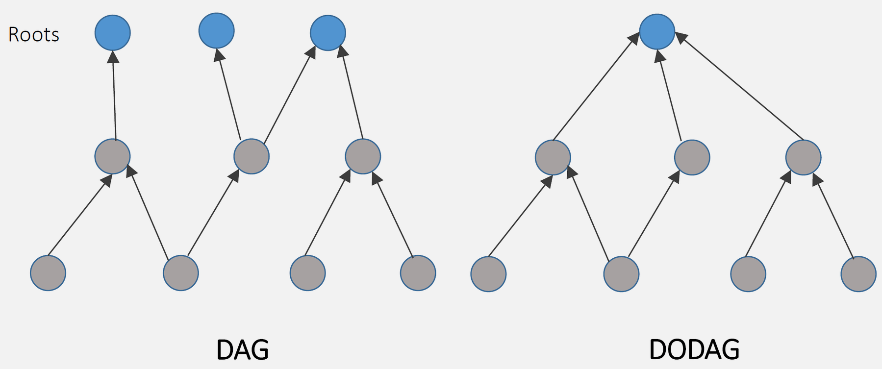
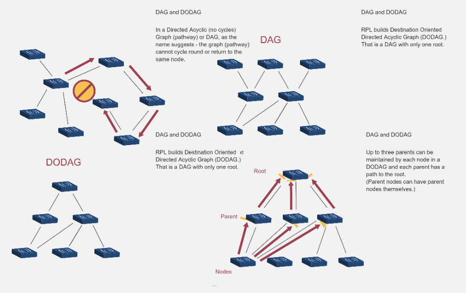
DODAG Properties: - Single root: One destination (typically border router/gateway) - Upward routes: All paths lead to root - RANK: Position in DODAG hierarchy (root = 0, increases going down)

708.5.3 RANK: Loop Prevention Mechanism

RANK is a scalar representing a node’s position relative to the root.

%%{init: {'theme': 'base', 'themeVariables': { 'primaryColor': '#2C3E50', 'primaryTextColor': '#fff', 'primaryBorderColor': '#16A085', 'lineColor': '#16A085', 'secondaryColor': '#E67E22', 'tertiaryColor': '#7F8C8D'}}}%%
graph TB
    ROOT["ROOT<br/>RANK = 0"]
    A["Node A<br/>RANK = 100"]
    B["Node B<br/>RANK = 250"]
    C["Node C<br/>RANK = 370"]

    ROOT -->|"Good link<br/>+100"| A
    A -->|"Poor link<br/>+150"| B
    B -->|"Good link<br/>+120"| C

    C -.->|"Cannot choose<br/>(370 > 100 = loop!)"| A

    style ROOT fill:#2C3E50,stroke:#16A085,color:#fff,stroke-width:4px
    style A fill:#16A085,stroke:#2C3E50,color:#fff
    style B fill:#E67E22,stroke:#2C3E50,color:#fff
    style C fill:#7F8C8D,stroke:#2C3E50,color:#fff

Figure 708.8: RPL RANK mechanism preventing routing loops by enforcing increasing rank away from root

{fig-alt=“RANK loop prevention mechanism showing ROOT at Rank 0, Node A at 100, B at 250, C at 370, with valid forward links and forbidden backward link from C to A that would create a loop”}

Figure 708.9: RPL RANK mechanism preventing loops by increasing rank with distance from root

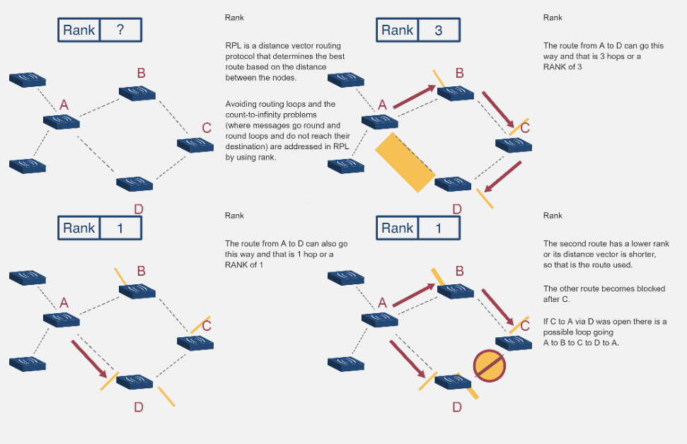
RANK Rules: 1. Root has RANK 0 (or minimum RANK) 2. RANK increases as you move away from root 3. Upward routing: Packets forwarded to nodes with lower RANK 4. Loop prevention: Node cannot choose parent with higher RANK

RANK Calculation:

RANK(node) = RANK(parent) + RankIncrease

RankIncrease calculated based on:
- Link cost (ETX, RSSI, etc.)
- Number of hops
- Energy consumed
- Objective function

Example:

ROOT: RANK = 0
Node A (parent: ROOT): RANK = 0 + 100 = 100
Node B (parent: Node A): RANK = 100 + 150 = 250
Node C (parent: Node B): RANK = 250 + 120 = 370

Loop Prevention: - Node C cannot choose Node A as parent (RANK 100 < 370 is OK) - Node A cannot choose Node C as parent (RANK 370 > 100 - would create loop)

ImportantRANK vs Hop Count

RANK is not the same as Hop Count (although hop count can be a factor)

RANK is calculated using objective function which may consider: - Hop count - Expected Transmission Count (ETX) - Latency - Energy consumption - Link quality (RSSI, LQI)

Example: - Good link, 1 hop: RANK increase = 100 - Poor link, 1 hop: RANK increase = 300 - Good link, 2 hops: RANK increase = 200

Node may prefer 2 hops via good links (total RANK increase: 200) over 1 hop via poor link (RANK increase: 300).

---

708.6 What’s Next

Now that you understand RPL’s core concepts—DODAG topology, RANK mechanism, and why traditional protocols don’t work for IoT—the next chapter covers how RPL actually builds the DODAG and the two operational modes.

Continue to: RPL DODAG Construction and Modes

• DODAG construction process step-by-step
• DIO, DIS, DAO control messages
• Storing mode vs Non-Storing mode comparison
• Memory and performance trade-offs