702 RPL Worked Example: Smart Lighting Network

702.1 Worked Example: DODAG Construction Step-by-Step

Learning Objectives

By the end of this section, you will be able to:

Calculate RANK values using actual RPL parameters
Perform parent selection with multiple candidate parents
Apply objective function formulas to real network scenarios
Interpret final DODAG structure for routing decisions

10-Node Smart Lighting Network

This worked example walks through the complete DODAG construction process for a realistic smart lighting deployment. We will calculate RANK values using actual RPL parameters and show how parent selection works with varying link qualities.

702.2 Problem Context

Scenario: You are deploying a smart lighting mesh network in a commercial building lobby. The network consists of:

1 Border Router (Root): Connected to the building management system
9 Smart Light Controllers: Need to report status and receive dimming commands
Goal: Build an RPL DODAG for reliable many-to-one (sensor data) and one-to-many (commands) communication

702.3 Given Parameters

RPL Configuration (RFC 6550 defaults):

Parameter	Value	Description
MinHopRankIncrease	256	Minimum RANK increase per hop
Objective Function	OF0 with ETX	Minimize Expected Transmission Count
ETX Calculation	ETX = 1 / (delivery_ratio)	Higher ETX = worse link
RANK Formula	RANK = Parent_RANK + (MinHopRankIncrease x ETX)	Cumulative path cost

Network Topology and Link Quality:

{fig-alt=“10-node smart lighting network topology showing border router ROOT at top connected to first-hop nodes A B C, which connect to second-hop nodes D E F, which connect to third-hop leaf nodes G H I. Links labeled with ETX values ranging from 1.0 for good links to 2.0 for poor links, demonstrating varying wireless link quality in building environment”}

702.4 Solution: Step-by-Step DODAG Construction

702.4.1 Step 1: Root Advertisement (t = 0s)

Root Action: Border router initializes DODAG and broadcasts first DIO message.

DIO Message Contents:

DIO {
  DODAG_ID: fd00::1
  RANK: 0
  Version: 1
  MinHopRankIncrease: 256
  Objective Function: OF0 (ETX)
}

Result: Root has RANK = 0. All nodes within radio range receive this DIO.

702.4.2 Step 2: First-Hop Nodes Calculate RANK (t = 2-5s)

Nodes A, B, and C receive the root’s DIO and calculate their RANK values:

Node A Calculation: \[\text{RANK}_A = \text{Parent\_RANK} + (\text{MinHopRankIncrease} \times \text{ETX})\] \[\text{RANK}_A = 0 + (256 \times 1.0) = \mathbf{256}\]

Node B Calculation: \[\text{RANK}_B = 0 + (256 \times 1.0) = \mathbf{256}\]

Node C Calculation: \[\text{RANK}_C = 0 + (256 \times 1.5) = \mathbf{384}\]

Parent Selection: All three nodes select ROOT as parent (only option).

Node	Parent	ETX to Parent	Calculated RANK
A	ROOT	1.0	256
B	ROOT	1.0	256
C	ROOT	1.5	384

Actions: 1. Each node sends DAO to ROOT announcing reachability 2. Each node broadcasts DIO with its new RANK to neighbors

702.4.3 Step 3: Second-Hop Nodes - Parent Selection Decision (t = 5-10s)

This is where RPL’s intelligence shines. Second-hop nodes may hear DIOs from multiple parents and must choose the best one.

Node D: Receives DIO only from Node A \[\text{RANK}_D = 256 + (256 \times 1.0) = \mathbf{512}\] - Parent: A (only option)

Node E: Receives DIOs from both A and B (key decision point!)

Option 1: Via Node A (ETX 1.5) \[\text{RANK}_E^{(A)} = 256 + (256 \times 1.5) = 640\]

Option 2: Via Node B (ETX 1.0) \[\text{RANK}_E^{(B)} = 256 + (256 \times 1.0) = \mathbf{512}\]

Decision: Node E selects B as primary parent (lower RANK = better path) - Node E also stores A as backup parent (RANK 640, valid alternate)

Node F: Receives DIOs from B and C

Option 1: Via Node B (ETX 1.0) \[\text{RANK}_F^{(B)} = 256 + (256 \times 1.0) = \mathbf{512}\]

Option 2: Via Node C (ETX 1.5) \[\text{RANK}_F^{(C)} = 384 + (256 \times 1.5) = 768\]

Decision: Node F selects B as primary parent (RANK 512 < 768)

Node	Candidate Parents	Calculated RANKs	Selected Parent	Final RANK
D	A only	512	A	512
E	A (640), B (512)	640, 512	B	512
F	B (512), C (768)	512, 768	B	512

Key Insight: Link Quality Trumps Hop Count

Notice that Node F could reach ROOT via C in just 2 hops (F to C to ROOT), but the poor link quality (ETX 1.5 + 1.5) makes this path worse than going through B (ETX 1.0 + 1.0), even though both are 2 hops. RANK incorporates link quality, not just hop count.

702.4.4 Step 4: Third-Hop Nodes - Final RANK Calculation (t = 10-15s)

Node G: Receives DIOs from D and E

Option 1: Via Node D (ETX 1.0) \[\text{RANK}_G^{(D)} = 512 + (256 \times 1.0) = \mathbf{768}\]

Option 2: Via Node E (ETX 2.0 - poor link!) \[\text{RANK}_G^{(E)} = 512 + (256 \times 2.0) = 1024\]

Decision: Node G selects D as parent (768 < 1024)

Node H: Receives DIOs from E and F

Option 1: Via Node E (ETX 1.0) \[\text{RANK}_H^{(E)} = 512 + (256 \times 1.0) = \mathbf{768}\]

Option 2: Via Node F (ETX 1.5) \[\text{RANK}_H^{(F)} = 512 + (256 \times 1.5) = 896\]

Decision: Node H selects E as parent (768 < 896)

Node I: Receives DIO only from F \[\text{RANK}_I = 512 + (256 \times 1.0) = \mathbf{768}\] - Parent: F (only option)

Node	Candidate Parents	Calculated RANKs	Selected Parent	Final RANK
G	D (768), E (1024)	768, 1024	D	768
H	E (768), F (896)	768, 896	E	768
I	F only	768	F	768

702.4.5 Step 5: DAO Propagation - Building Downward Routes (t = 15-25s)

After DODAG formation, DAO messages flow upward to build downward routing tables:

{fig-alt=“DAO message propagation sequence showing Node G sending DAO to parent D announcing reachability, D aggregating and sending to A, A aggregating and sending to ROOT. Each intermediate node stores routing entries. ROOT confirms with DAO-ACK flowing back down through D and A to G, completing downward route establishment”}

702.4.6 Step 6: Final DODAG Structure (t = 25-30s)

{fig-alt=“Final DODAG structure for 10-node smart lighting network showing hierarchical tree rooted at border router with Rank 0. First hop has nodes A B C with Ranks 256 256 384. Second hop has D E F all with Rank 512, where B serves as parent for both E and F. Third hop has leaf nodes G H I all with Rank 768. Dotted lines show backup parent relationships from A to E and F to H for fault tolerance”}

702.5 Final Answer: Complete RANK Summary

Node	Layer	Parent	ETX to Parent	RANK Calculation	Final RANK
ROOT	0	-	-	Root node	0
A	1	ROOT	1.0	0 + 256x1.0	256
B	1	ROOT	1.0	0 + 256x1.0	256
C	1	ROOT	1.5	0 + 256x1.5	384
D	2	A	1.0	256 + 256x1.0	512
E	2	B	1.0	256 + 256x1.0	512
F	2	B	1.0	256 + 256x1.0	512
G	3	D	1.0	512 + 256x1.0	768
H	3	E	1.0	512 + 256x1.0	768
I	3	F	1.0	512 + 256x1.0	768

702.6 Interpretation: How RANK Determines Routing

Upward Routing (Sensor Data to Cloud): - Each node simply forwards to its parent (follows decreasing RANK) - Example: Light #9 (Node I) sends status: I to F (512) to B (256) to ROOT (0) to Cloud - Total path cost: 768 (Node I’s RANK represents cumulative ETX)

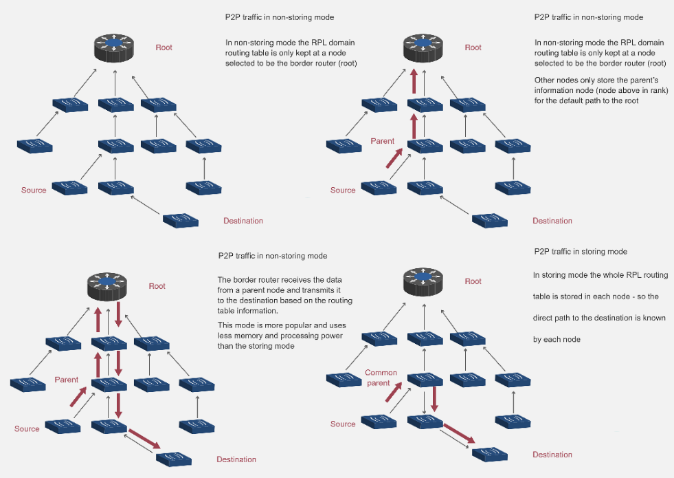
Downward Routing (Commands to Lights): - ROOT uses stored routing table from DAO messages - Example: Dim command to Light #7 (Node G): ROOT to A to D to G - Source routing header (Non-Storing) or hop-by-hop lookup (Storing)

Loop Prevention: - Data only flows toward lower RANK (upward) or via explicit routes (downward) - Node E (RANK 512) cannot send to Node F (RANK 512) directly - Point-to-point: E to B (256) to F (512) via common ancestor

Fault Tolerance: - If Node B fails, E has backup parent A (RANK 640 > 512, but functional) - E would recalculate: RANK_E = 256 + 384 = 640, network continues operating - Trickle timer detects failure within 3-4 DIO intervals

Key Takeaways from This Example

RANK is cumulative: Each hop adds MinHopRankIncrease x ETX, not just +1
Link quality matters: Node F chose B over C despite C being available, because B offered better cumulative path quality
Multiple parents: Nodes can maintain backup parents for resilience (A as backup for E)
Unbalanced trees are OK: Node B has 3 descendants (E, F, H, I indirectly), while C has none - this is optimal given link quality
RANK inversion = loop: If Node H somehow got RANK < 512, it would create a loop with E - RPL prevents this
MinHopRankIncrease = 256: This standard value allows for 16 sub-levels (256/16=16) of rank differentiation per hop for fine-grained path selection

702.7 Detailed Construction Steps

Step 1: Root Initiates DODAG

Root node (border router/gateway): 1. Creates DODAG: Assigns unique DODAG ID 2. Sets RANK = 0: Root has minimum RANK 3. Broadcasts DIO: Sends DODAG Information Object (multicast)

DIO Contents: - DODAG ID (IPv6 address) - RANK (0 for root) - Objective function (routing metric) - DODAG configuration (timers, etc.)

Four-stage RPL DODAG formation process showing temporal progression: stage 1 root node initializes DODAG and broadcasts first DIO messages, stage 2 first-hop neighbor nodes receive DIOs and calculate RANK values to join as direct children, stage 3 second-hop nodes receive propagated DIOs from first-hop nodes and establish parent relationships, stage 4 complete DODAG topology with all nodes organized in hierarchical layers by RANK distance from root — Figure 702.4: RPL DODAG construction steps from root initialization to completion

702.8 Step 2: Nodes Receive DIO and Join

Node receives DIO: 1. Decision: Join this DODAG or wait for others? - Compare DODAG rank, objective function - May receive DIOs from multiple DODAGs 2. Calculate RANK: RANK = parent_RANK + increase 3. Select parent: Choose sender of DIO (if acceptable) 4. Update state: Store DODAG ID, parent, RANK

Multiple DIO Sources: - Node may hear DIOs from multiple neighbors - Chooses best parent (lowest RANK, best link quality) - May maintain backup parents (loop-free)

Quiz 1: Step 2: Nodes Receive DIO and Join

Question 7: An agricultural IoT network using RPL experiences a node failure. Node D was the parent for three child nodes (E, F, G). What happens during network self-healing?

Explanation: RPL’s self-healing is distributed and automatic. Each node expects periodic DIO messages from its parent. When nodes E, F, G stop receiving DIOs from D (typically after 3-4 missed intervals based on trickle timer), they: 1. Mark parent D as unreachable 2. Select new best parent from cached DIO information of other neighbors 3. Update their RANK based on new parent 4. Send updated DAO messages (in Storing mode) to advertise their reachability via new path 5. Resume normal operation

This process is local - no global reconstruction needed. The trickle timer algorithm balances responsiveness (fast recovery) with efficiency (infrequent messages when network is stable). DIS messages can accelerate discovery but aren’t required. Global reconstruction only occurs for major events (root failure, DODAG version increment).

Question 10: A battery-powered soil moisture sensor network uses RPL with 50 nodes over 15 km squared. Nodes are 3-7 hops from the root. What RPL optimization would most significantly extend battery life?

Explanation: For battery-powered sensor networks with primarily many-to-one traffic (sensors to gateway), the biggest energy drain is control message overhead (DIO, DAO transmissions). Optimization A addresses this: - Non-Storing mode: No DAO messages propagating between nodes (only to root), reducing TX overhead - Trickle timer: RPL’s adaptive timer sends DIOs frequently when network changes, but exponentially backs off to very infrequent transmissions (minutes/hours) when stable. Aggressive suppression means nodes listen for redundant DIOs and skip their own transmission if neighbors already sent

Why not others: - B (Storing mode): Increases DAO overhead; P2P traffic is rare in sensor networks - C (Disable DAO): Breaks downward routing; needed for configuration updates - D (More DIOs): Increases energy consumption, opposite of goal

Energy calculation: In stable network, trickle timer can reduce DIOs from every 10s to every 1 hour, saving 360x transmissions!

702.9 Step 3: Nodes Propagate DIO

After joining DODAG: 1. Node becomes part of DODAG 2. Sends own DIO: Advertises DODAG to neighbors 3. DIO contents: Own RANK, DODAG ID, etc. 4. Trickle timer: Controls DIO frequency (adaptive)

Trickle Algorithm: - Stable network: Send DIOs infrequently (minutes) - Network changes: Send DIOs frequently (seconds) - Reduces overhead while maintaining responsiveness

Step 4: Build Upward Routes

Upward routes (towards root) established automatically: - Each node knows its parent (from DIO selection) - Default route: Send to parent (towards root) - No routing table needed for upward routes (just parent pointer)

Example:

Node 3 -> Node 1 -> Root
(N3 knows parent is N1, N1 knows parent is Root)

Step 5: Build Downward Routes (Storing Mode)

Downward routes (from root to nodes) require DAO messages:

Node sends DAO to parent:
- “I am reachable via you”
- Includes node’s address and prefixes
Parent updates routing table:
- “Node X is reachable via this child”
Parent propagates DAO towards root:
- Aggregates reachability information
Root knows all nodes:
- Complete routing table for downward routes

DAO-ACK (optional): - Parent confirms DAO receipt - Reliability for critical networks

Quiz 2: Step 5: Build Downward Routes (Storing Mode)

Question 3: A parking sensor network uses RPL in Storing mode. Sensor A (RANK 5) needs to send data to Sensor B (RANK 6). How is this point-to-point traffic routed?

Explanation: In Storing mode, each node maintains routing tables populated by DAO messages. When Sensor A needs to reach Sensor B, it looks up B’s address in its routing table and forwards the packet accordingly. The routing may go through intermediate nodes, but doesn’t necessarily go through the root. This is the key advantage of Storing mode for P2P traffic - direct/optimized paths. In Non-Storing mode, the packet would go up to the root, which then source-routes it down to B. Storing mode trades memory (routing tables) for lower P2P latency.

702.10 Summary

This worked example demonstrated:

RANK Calculation: Using MinHopRankIncrease x ETX formula to compute cumulative path cost
Parent Selection: Comparing multiple candidate parents and choosing the one offering lowest RANK
Link Quality Impact: How poor links (high ETX) cause nodes to prefer longer paths with better quality
Backup Parents: Maintaining alternate routes for fault tolerance
Routing Interpretation: How RANK determines upward, downward, and point-to-point routing paths

702.11 What’s Next

Continue to RPL Trickle Algorithm and Routing Modes to learn how the Trickle timer minimizes control overhead and understand the trade-offs between Storing and Non-Storing modes.