701 RPL Trickle Algorithm and Routing Modes

701.1 Trickle Algorithm and Routing Modes

Learning Objectives

By the end of this section, you will be able to:

Understand the Trickle algorithm for adaptive control message timing
Compare Storing mode vs Non-Storing mode trade-offs
Design RPL networks for different IoT applications
Analyze RPL performance trade-offs for traffic patterns

701.2 Understanding Trickle: The “Polite Gossip” Protocol

The Trickle algorithm is RPL’s secret weapon for efficient network-wide consistency. Think of it as a polite conversation at a party:

The Party Metaphor: How Trickle Works

Imagine you’re at a party where everyone should know the same information (like when dinner is served):

The Social Dynamics:

At a party, if everyone says the same thing (consistent state), you stay quiet. But if you hear something different (inconsistency), you speak up. Over time, conversation naturally decreases as consensus forms.

The Five Rules of Polite Gossip:

Listen first: When you arrive, listen to what others are saying (gather neighbor DIOs)
Stay quiet if consistent: If everyone’s saying the same thing, no need to repeat (suppress transmission)
Speak up if different: If you hear something wrong, correct it immediately (reset interval on inconsistency)
Gradually relax: As consensus forms, conversations naturally decrease (double interval on stability)
Reset on news: When new information arrives, the buzz picks up again (interval reset)

This is exactly how RPL nodes behave when spreading DODAG information!

Technical Mapping: Party to Network:

Party Element	Trickle Mechanism	Technical Detail
Party	RPL Network	DODAG topology
Gossip	DIO messages	DODAG Information Objects
Same story	Consistent state	Same DODAG Version, RANK, parent
Different story	Inconsistency	New Version, RANK change, topology change
Listen period	Interval timer `I`	Current interval: Imin <= I <= Imax
Counter	Consistency counter `c`	How many consistent DIOs heard
Threshold	Redundancy constant `k`	Suppress if c >= k
Speak up	Broadcast DIO	Share DODAG information
Stay quiet	Suppress transmission	Save energy when c >= k
Conversation dying down	Double interval	I = min(2xI, Imax)
New gossip	Reset interval	I = Imin on inconsistency

How Trickle Achieves Efficiency:

{fig-alt=“Trickle algorithm state machine showing Listen phase collecting neighbor DIOs, CheckConsistency evaluating if counter threshold k is met, branching to Suppress (save energy), Broadcast (maintain awareness), or Inconsistent (urgent update), followed by DoubleInterval for stable networks or ResetInterval for network changes, creating adaptive control message frequency”}

Academic Resource: Trickle Execution Example

The Cambridge Mobile and Sensor Systems course demonstrates Trickle timing with a 3-node example using redundancy threshold k=1:

Timeline Analysis:

Time	Node 1	Node 2	Node 3	Action
t=0	c=0	c=0	c=0	All start listening
t1a	TX	-	-	Node 1 transmits (c=0 < k=1)
t1a-all	-	c=1	c=1	Nodes 2,3 increment c on reception
t2a	-	SUPPRESS	-	Node 2 suppresses (c=1 >= k=1)
t2b	-	-	SUPPRESS	Node 3 suppresses (c=1 >= k=1)
interval x 2	-	-	-	All nodes double interval (stable)

Key Insight: When k=1, nodes suppress transmission after hearing just one consistent message from a neighbor. This exponentially reduces overhead while maintaining network awareness.

Source: University of Cambridge - Mobile and Sensor Systems (Prof. Cecilia Mascolo)

701.3 Trickle Timer Behavior: The Three Scenarios

Scenario 1: Stable Network (Doubling Interval)

What happens: Everyone at the party is saying the same thing, so conversation naturally dies down.

Technical behavior: - Node starts interval I = Imin (e.g., 10s) - During listening period, hears k or more consistent DIOs from neighbors - Suppresses transmission (stays quiet) - Doubles interval: I = min(2xI, Imax) - Next interval: 10s to 20s to 40s to 80s to … to 1 hour

Example timeline:

t=0s:    I=10s,  Heard 5 DIOs (all RANK=100), Suppress, Next I=20s
t=20s:   I=20s,  Heard 4 DIOs (all RANK=100), Suppress, Next I=40s
t=60s:   I=40s,  Heard 3 DIOs (all RANK=100), Suppress, Next I=80s
t=140s:  I=80s,  Heard 2 DIOs (all RANK=100), Suppress, Next I=160s
...
t=3600s: I=3600s (1 hour), Heard 1 DIO, Suppress, Stay at I=3600s (Imax)

Energy savings: After 10 doublings, a node that would have sent 360 DIOs/hour now sends just 1 DIO/hour = 360x reduction!

Scenario 2: Network Inconsistency (Reset Interval)

What happens: Someone says something different at the party—everyone starts talking to correct it!

Technical behavior: - Node hears DIO with different DODAG information: - Different DODAG Version Number - Parent changed RANK - New Objective Function - Immediately broadcasts DIO to share correct information - Resets interval: I = Imin (back to minimum) - Counter resets: c = 0 - Network rapidly converges to new consistent state

Example timeline:

t=0s:     I=3600s (stable at 1 hour interval)
t=100s:   INCONSISTENCY DETECTED! Parent RANK changed 100->150
          -> Broadcast DIO immediately
          -> Reset I=10s (Imin)
          -> Reset counter c=0

t=110s:   I=10s,  Heard 6 DIOs (all consistent with new RANK), Suppress, I=20s
t=130s:   I=20s,  Heard 5 DIOs (consistent), Suppress, I=40s
t=170s:   I=40s,  Heard 4 DIOs (consistent), Suppress, I=80s
...
(Network re-stabilizes and returns to hourly DIOs)

Why this matters: Topology changes propagate in seconds (multiple nodes reset timers), but stable network returns to hourly updates = responsive yet efficient!

Scenario 3: Insufficient Redundancy (Broadcast)

What happens: Not enough people are talking at the party—you chime in to maintain awareness.

Technical behavior: - Node hears fewer than k consistent DIOs during interval - Counter c < k (e.g., c=1, k=3) - Broadcasts DIO to ensure information dissemination - Doubles interval normally: I = min(2xI, Imax) - Ensures at least k nodes transmit per interval (redundancy)

Example scenario:

Sparse network area (only 2 neighbors):

t=0s:   I=10s,  Heard 1 DIO (c=1 < k=3), BROADCAST DIO, Next I=20s
t=20s:  I=20s,  Heard 2 DIOs (c=2 < k=3), BROADCAST DIO, Next I=40s
t=60s:  I=40s,  Heard 2 DIOs (c=2 < k=3), BROADCAST DIO, Next I=80s

Network edge behavior: Nodes at DODAG edges (fewer neighbors) broadcast more frequently to maintain connectivity, while dense core suppresses aggressively.

701.4 Why Trickle Saves Energy in Stable Networks

The genius of Trickle is exponential backoff combined with instant reset:

Energy math: - Periodic DIO (no Trickle): Send every 10s = 360 DIOs/hour = 360 transmissions - Trickle (stable network): Send every 1 hour = 1 DIO/hour = 1 transmission - Savings: 99.7% reduction in control overhead!

Real-world battery impact:

{fig-alt=“Trickle energy savings diagram comparing 360 DIOs/hour without Trickle (16.2 mAh/hour) vs 1 DIO/hour with Trickle (0.045 mAh/hour), showing 99.7% reduction and 141.6 Ah/year saved, extending battery life by 5-10 months”}

Assumptions: 5mA transmit current, 3ms transmission time, 2000mAh battery

Why This Matters for IoT:

The Trickle algorithm enables RPL to achieve network-wide consistency with minimal energy expenditure:

Stable network (99% of the time): Nodes send DIOs every 10-60 minutes, conserving battery
Network change (1% of the time): Nodes send DIOs every 10-500ms for rapid convergence
Polite suppression: If 5 neighbors already broadcasted the same DIO, no need to add redundancy
Instant reaction: Inconsistency (e.g., RANK change, parent failure) triggers immediate reset to fast interval

Real-world impact: In a 100-node smart building, Trickle reduces DIO overhead from ~600,000 messages/day (periodic every 10s) to ~14,400 messages/day (adaptive, mostly hourly), extending battery life by 41x while maintaining sub-minute response to topology changes.

RFC 6206 Parameters: - Imin: Minimum interval (10ms-1s) - fast response to changes - Imax: Maximum interval (1min-1hr) - low overhead when stable - k: Redundancy constant (2-8) - consistency threshold before suppression - c: Listen-only period (0-50% of interval) - gather info before deciding

701.5 Trickle Algorithm: Visual Explanation

Trickle is “polite gossip” - nodes share information only when needed.

701.5.1 The Algorithm in 4 Steps

{fig-alt=“Trickle algorithm 4-step visual flowchart showing Step 1 (navy) initializing interval I to Imin, resetting counter c to 0, and picking random transmission time t; Step 2 (teal) listening for consistent information and incrementing counter; Step 3 (orange) decision point checking if counter c is less than redundancy constant k, branching to Transmit if yes or Stay Silent if no; Step 4 (navy) doubling the interval up to Imax and restarting the cycle, demonstrating adaptive control message frequency for RPL networks”}

701.5.2 Key Parameters

Parameter	Meaning	Typical Value
Imin	Minimum interval (fast response)	100ms
Imax	Maximum interval (energy saving)	16 minutes
k	Redundancy constant (suppression threshold)	1-5
c	Consistency counter (heard transmissions)	Incremented per consistent message
t	Random transmission time in [I/2, I]	Prevents collisions

701.5.3 Why Trickle Works

Consistent network: Everyone agrees, intervals grow exponentially, minimal traffic
Inconsistency detected: Reset interval to Imin, quick resync across network
New node joins: Hears inconsistent info, triggers rapid updates from neighbors
Suppression: If enough neighbors already transmitted (c >= k), stay silent to save energy

701.6 RPL Routing Modes

RPL supports two modes with different memory/performance trade-offs:

701.6.1 Storing Mode

Each node maintains routing table for its sub-DODAG.

{fig-alt=“RPL Storing mode showing distributed routing tables: ROOT maintains routes to all nodes, intermediate nodes B and C maintain routes to their descendants, enabling distributed forwarding decisions”}

RPL storing mode diagram illustrating distributed routing architecture where each node maintains a routing table containing downward routes to its descendant nodes populated by DAO messages, enabling intermediate nodes to make independent forwarding decisions and route packets directly to destinations within their sub-DODAG without requiring root node involvement, supporting efficient point-to-point communication with optimal path selection — RPL Modes of Operation

Artistic visualization of RPL storing mode operation showing the distributed routing architecture with color-coded nodes indicating rank levels, parent-child relationships depicted with directional arrows, routing table contents displayed within each node box, and data flow patterns illustrated to demonstrate how storing mode enables efficient point-to-point routing without requiring all traffic to pass through the root node. — RPL Modes of Operation

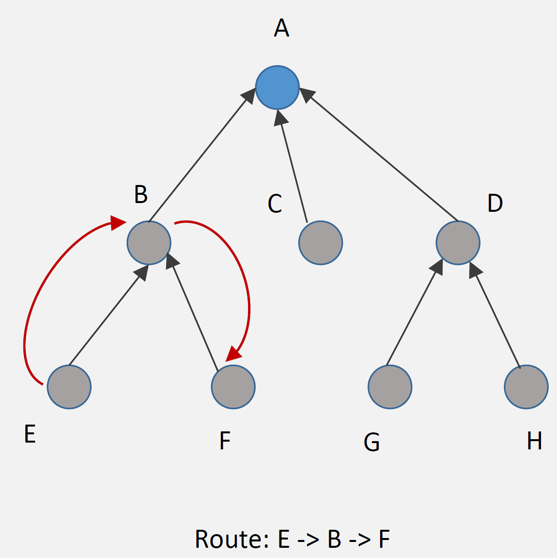
How It Works: 1. DAO messages: Nodes advertise reachability to parents 2. Routing tables: Each node stores routes to descendants 3. Packet forwarding: Node looks up destination in table, forwards to appropriate child

Example Route (E to F):

Step 1: E sends packet to parent B (upward)
Step 2: B checks routing table: "F is my child"
Step 3: B forwards directly to F (downward)

Route: E -> B -> F (optimal)

Advantages: - Efficient routing: Optimal paths (no detour through root) - Low latency: Direct routes between any nodes - Root not bottleneck: Distributed routing decisions

Disadvantages: - Memory overhead: Each node stores routing table - Scalability: Routing tables grow with network size - Updates: DAO messages for every node change

Best For: - Devices with sufficient memory (32+ KB RAM) - Networks requiring low latency - Point-to-point communication common

701.6.2 Non-Storing Mode

Only root maintains routing information; exploits source routing.

{fig-alt=“RPL Non-Storing mode showing centralized routing at ROOT with complete topology, intermediate nodes maintain only parent pointers, downward routing uses source routing headers from root”}

RPL non-storing mode diagram illustrating centralized routing architecture where only the root node maintains complete network topology information collected via DAO messages sent directly to root, intermediate nodes store only parent pointers for upward routing, all downward traffic must route through root which inserts source routing headers specifying complete hop-by-hop paths, minimizing memory requirements on constrained nodes at the cost of suboptimal routing paths and increased root processing load — RPL Non-Storing Mode Operation

Artistic visualization of RPL non-storing mode showing centralized routing architecture where the root node is prominently displayed with complete topology knowledge, intermediate nodes shown as lightweight with only parent pointers, source routing headers visualized as path specifications embedded in packets flowing downward, demonstrating the trade-off between memory efficiency on constrained nodes and suboptimal routing paths through the root. — RPL Non-Storing Mode Operation

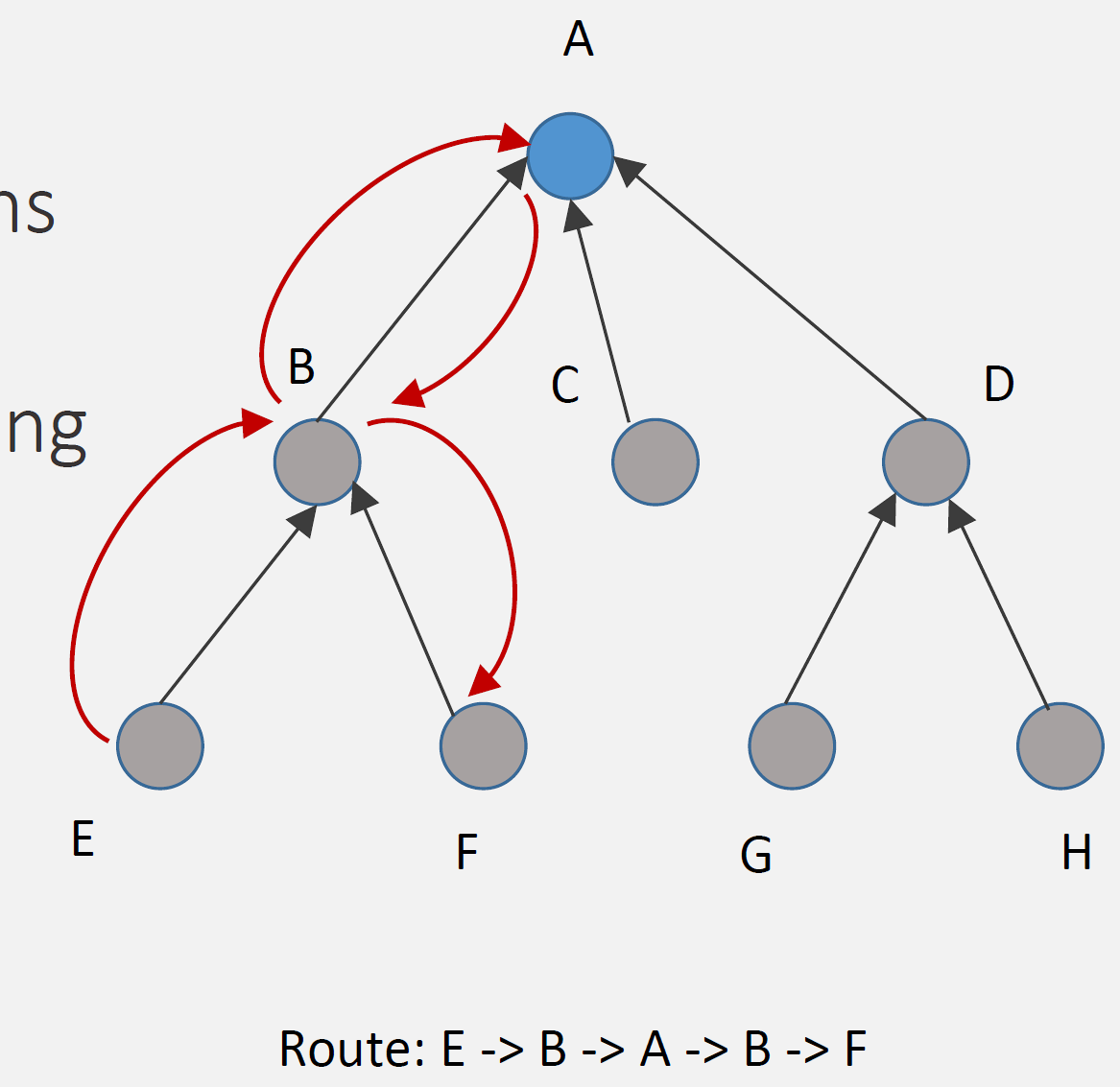
How It Works: 1. DAO to root: All nodes send DAO directly to root (upward) 2. Root stores all routes: Only root has complete routing table 3. Source routing: Root inserts complete path in packet header 4. Nodes forward: Follow instructions in packet header (no table lookup)

Example Route (E to F):

Step 1: E sends packet to parent B (upward, default route)
Step 2: B forwards to parent A (root) (upward, default route)
Step 3: A (root) checks routing table: "F via B"
Step 4: A inserts source route: [B, F]
Step 5: A sends to B with route in header
Step 6: B forwards to F following route

Route: E -> B -> A -> B -> F (via root)

Advantages: - Low memory: Nodes don’t store routing tables (just parent) - Simple nodes: Minimal routing logic - Scalability: Network size doesn’t affect node memory

Disadvantages: - Suboptimal routes: All point-to-point traffic via root - Higher latency: Extra hops through root - Root bottleneck: All routing decisions at root - Header overhead: Source route in every packet

Best For: - Resource-constrained devices (< 16 KB RAM) - Primarily many-to-one traffic (sensors to gateway) - Point-to-point communication rare - Large networks (many nodes)

701.6.3 Storing vs Non-Storing Comparison

Aspect	Storing Mode	Non-Storing Mode
Routing Table	Distributed (all nodes)	Centralized (root only)
Node Memory	Higher (routing table)	Lower (parent pointer only)
Route Optimality	Optimal (direct paths)	Suboptimal (via root)
Latency	Lower	Higher (extra hops)
Root Load	Low	High (all routing decisions)
Scalability	Limited by node memory	Limited by root capacity
DAO Destination	Parent	Root (through parents)
Header Overhead	Low	High (source routing)
Best For	Powerful nodes, low latency	Constrained nodes, many-to-one

Quiz 3: RPL Routing Modes

Question 8: A factory monitoring network uses RPL with two instances: Instance 1 for high-priority safety alerts (latency metric) and Instance 2 for routine telemetry (energy metric). How does a node handle routing for different traffic types?

Explanation: RPL supports multiple instances on the same physical network, each with its own DODAG, root, and objective function. A node can simultaneously participate in Instance 1 (optimizing for latency) and Instance 2 (optimizing for energy), maintaining separate parent selections and RANK values. When forwarding a safety alert, the node uses Instance 1’s routing (e.g., parent with lowest latency path). For telemetry, it uses Instance 2’s routing (e.g., parent with best energy efficiency). Example: Instance 1 might select a 1-hop mains-powered parent (fast, high power), while Instance 2 selects a 3-hop battery-powered parent (slower, low power). This allows traffic differentiation without QoS complexity. Each instance has a unique RPLInstanceID (0-255).

701.7 RPL Traffic Patterns

RPL optimizes for different traffic directions:

{fig-alt=“RPL traffic patterns: Many-to-One shows multiple sensors sending to gateway (upward routing), One-to-Many shows gateway sending to multiple actuators (downward), Point-to-Point shows direct sensor to actuator communication”}

701.7.1 Many-to-One (Upward Routing)

Pattern: Many sensors to Single gateway/root

How: - Each node knows parent (from DODAG construction) - Default route: Send to parent (toward root) - No routing table needed (upward)

Example: Temperature sensors reporting to cloud

Sensor 3 -> Node 1 -> Root -> Internet -> Cloud
(Upward along DODAG tree)

Optimization: - Most common traffic in IoT (data collection) - Minimal state: Just parent pointer - Efficient: Direct path to root

701.7.2 One-to-Many (Downward Routing)

Pattern: Single controller to Many actuators

How: - Storing mode: Each node has routing table, forwards optimally - Non-storing mode: Root inserts source route, nodes follow

Example: Controller sends “turn off” to all lights

Root -> [Multicast or unicast to each light]

Modes: - Storing: Root to Node 1 to Light 3 (optimal) - Non-storing: Root inserts route [Node 1, Light 3]

701.7.3 Point-to-Point (P2P)

Pattern: Sensor to Actuator (peer-to-peer)

How: - Upward then downward (via common ancestor, often root) - Storing mode: May find shorter path - Non-storing mode: Always via root

Example: Motion sensor triggers light

Storing: Sensor 3 -> Node 1 -> Light 4 (3 hops, if both under Node 1)
Non-Storing: Sensor 3 -> Node 1 -> Root -> Node 2 -> Light 4 (4 hops)

701.8 Common Pitfalls

Common Pitfalls

1. Choosing the Wrong RPL Mode (Storing vs Non-Storing)

Mistake: Using Storing mode on severely memory-constrained nodes (e.g., 2KB RAM sensors), causing routing table overflow and network instability when nodes cannot store routes to all descendants
Why it happens: Storing mode provides more efficient point-to-point routing, so developers default to it without calculating memory requirements. Each routing entry requires ~20-40 bytes; a node with 50 descendants needs 1-2KB just for routing tables
Solution: Calculate your network’s memory budget before choosing modes. Use Non-Storing mode when: (1) nodes have <8KB RAM, (2) network depth exceeds 4-5 hops, or (3) point-to-point traffic is rare. In Non-Storing mode, all downward routes go through the root, which must have sufficient memory but leaf nodes stay lightweight. For hybrid needs, consider using Storing mode only for nodes with adequate memory

2. Aggressive Trickle Timer Settings Causing Network Storms

Mistake: Setting Trickle timer Imin too low (e.g., 100ms) or Imax too small (e.g., 4 doublings) in dense networks, causing constant DIO flooding that overwhelms the radio channel and drains batteries
Why it happens: Developers test with small networks (3-5 nodes) where aggressive timers converge quickly. In production deployments with 50+ nodes, the same settings cause every node to transmit DIOs simultaneously during network events
Solution: Start with conservative Trickle settings: Imin = 2-4 seconds, Imax = 16-20 doublings (giving maximum intervals of hours). For stable networks, RPL naturally reduces DIO frequency through Trickle’s exponential backoff. Only decrease timers if convergence time is unacceptable for your application. Monitor DIO message rates - if you see >1 DIO/minute/node in steady state, your Trickle parameters are too aggressive

3. Single DODAG Root Without Redundancy

Mistake: Deploying production RPL networks with only one border router as the DODAG root, creating a single point of failure where root failure disconnects the entire network from the Internet
Why it happens: RPL documentation focuses on single-root DODAGs for simplicity. Adding multiple roots requires understanding RPL instances, DODAG IDs, and root coordination, which adds deployment complexity
Solution: For production deployments, configure multiple border routers with the same DODAG ID but different root preferences. Use RPL’s multiple DODAG instance feature to provide backup paths. Alternatively, deploy redundant roots with different DODAG IDs and configure important nodes to join both. Monitor root health and implement automatic failover scripts that promote a secondary root if the primary becomes unreachable

701.9 Visual Reference Gallery

RPL and DODAG Visualizations

The following AI-generated diagrams provide additional perspectives on RPL routing concepts.

701.9.1 DODAG Construction Process

RPL DODAG construction process overview showing root initialization, DIO message propagation, parent selection, and rank assignment in low-power wireless mesh networks

Building A DODAG - Overview

DODAG construction step 1 showing root node broadcasting initial DIO message with rank 0 and objective function parameters to neighboring nodes

Building A DODAG - Step 1

DODAG construction step 2 showing first-tier nodes receiving DIO, calculating rank based on link quality, and selecting preferred parent toward root

Building A DODAG - Step 2

DODAG construction step 3 showing second-tier nodes joining network, computing rank through received DIO messages, and building routing tree

Building A DODAG - Step 3

DODAG construction step 4 showing network convergence with all nodes having assigned ranks and preferred parents forming loop-free topology

Building A DODAG - Step 4

DODAG construction step 5 showing DAO message flow for downward route establishment in storing mode RPL networks

Building A DODAG - Step 5

DODAG construction step 6 showing completed DODAG with bidirectional routing paths and maintenance through Trickle timer

Building A DODAG - Step 6

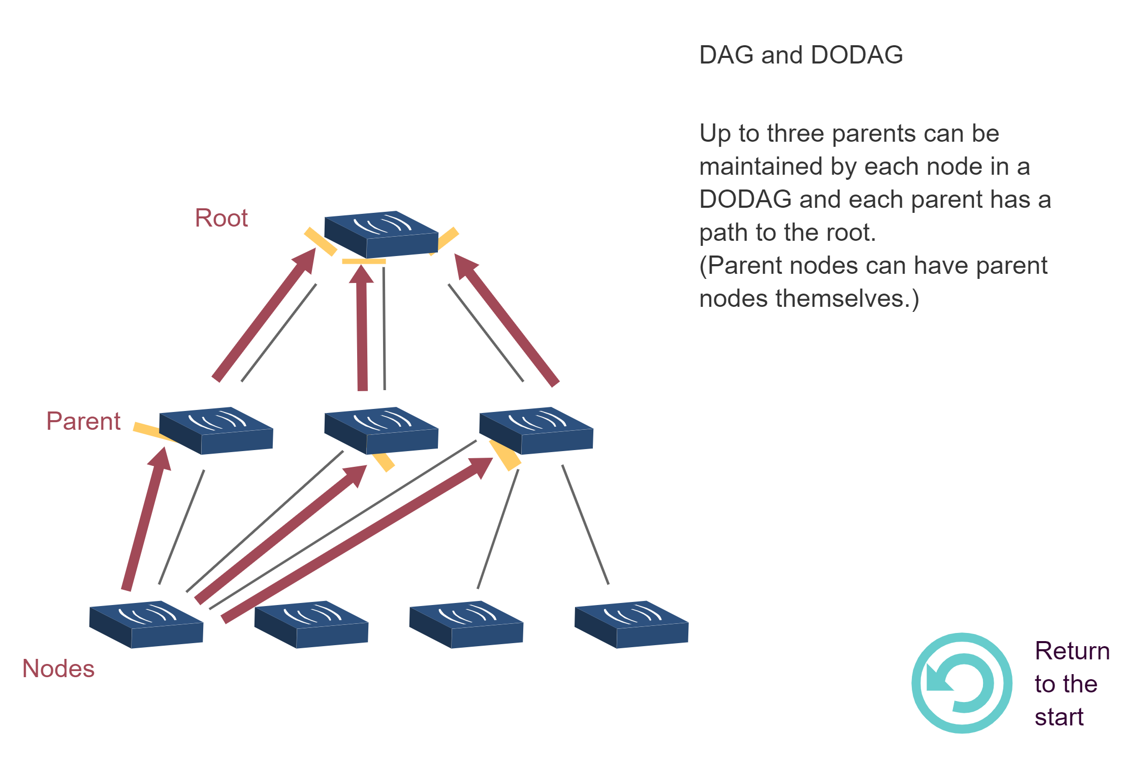
701.9.2 RPL Protocol Elements

RPL protocol fundamentals showing IPv6 routing protocol for LLNs with DODAG structure, control messages, and objective functions

RPL Protocol Overview 1

RPL control message types showing DIO, DIS, and DAO message formats with their roles in network formation and maintenance

RPL Protocol Overview 2

RPL objective functions showing ETX, hop count, and energy-aware metrics for path selection in wireless sensor networks

RPL Protocol Overview 3

RPL storing versus non-storing mode comparison showing memory requirements, routing paths, and suitable deployment scenarios

RPL Protocol Overview 4

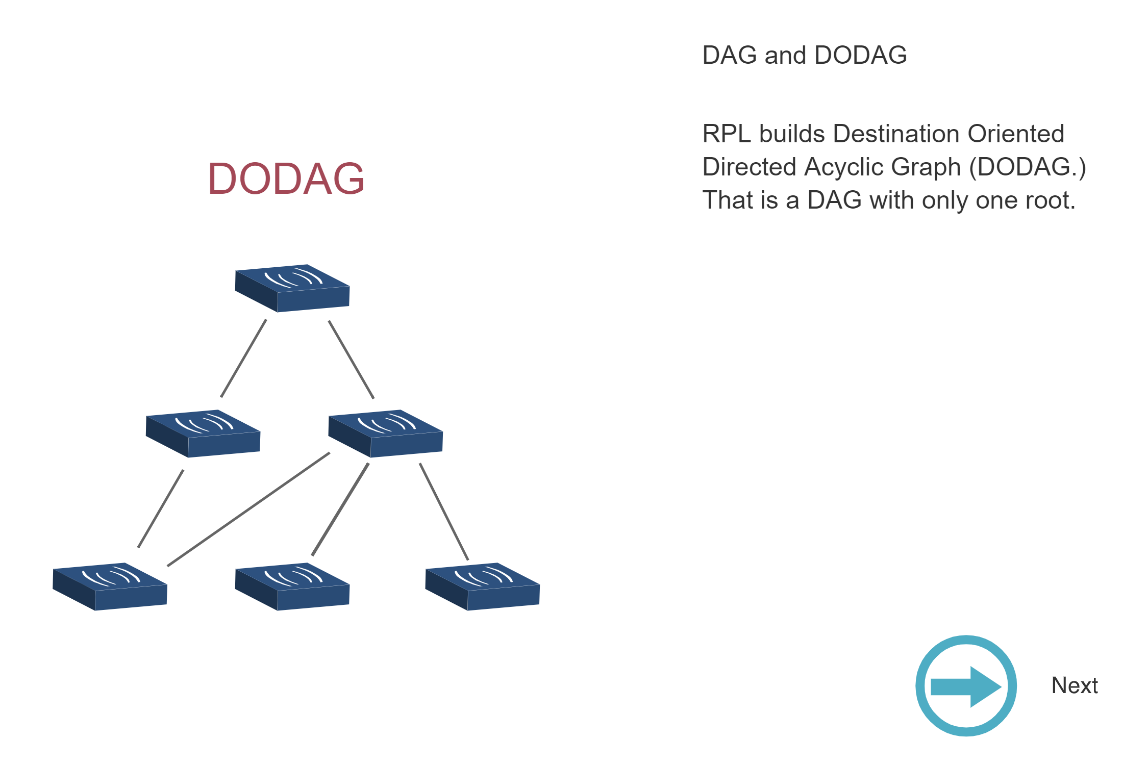
701.9.3 DODAG Structure

Difference between DAG and DODAG showing directed acyclic graph versus destination-oriented DAG with single root node

RPL DAG and DODAG 1

RPL DODAG instance showing multiple DODAGs coexisting with different roots for network redundancy and load balancing

RPL DAG and DODAG 2

RPL DODAG maintenance showing parent switching, rank updates, and loop detection mechanisms during network changes

RPL DAG and DODAG 3

Complete RPL DODAG construction sequence from root advertisement through network convergence with timing parameters

RPL DODAG Construction

RPL DODAG formation process showing Trickle timer operation, consistency checking, and message suppression for efficiency

RPL DODAG Formation

Detailed RPL DODAG formation showing DIO content, rank computation algorithm, and parent set maintenance

RPL DODAG Formation Detail

701.9.4 Rank Computation

RPL rank concept introduction showing hierarchical position value that increases away from root to prevent routing loops

RPL Rank 1

RPL rank computation showing MinHopRankIncrease, step values, and stretch factors for different objective functions

RPL Rank 2

RPL rank comparison showing how nodes select preferred parent based on advertised rank and link quality metrics

RPL Rank 3

RPL rank update scenarios showing rank increase, decrease constraints, and impact on network stability

RPL Rank 4

701.9.5 Applications

Smart building IoT deployment using RPL routing showing sensors, actuators, border router, and building management system integration

Smart Building with RPL

701.10 Original Source Figures (Alternative Views)

The following figures from the CP IoT System Design Guide provide alternative visual representations of RPL concepts covered in this chapter.

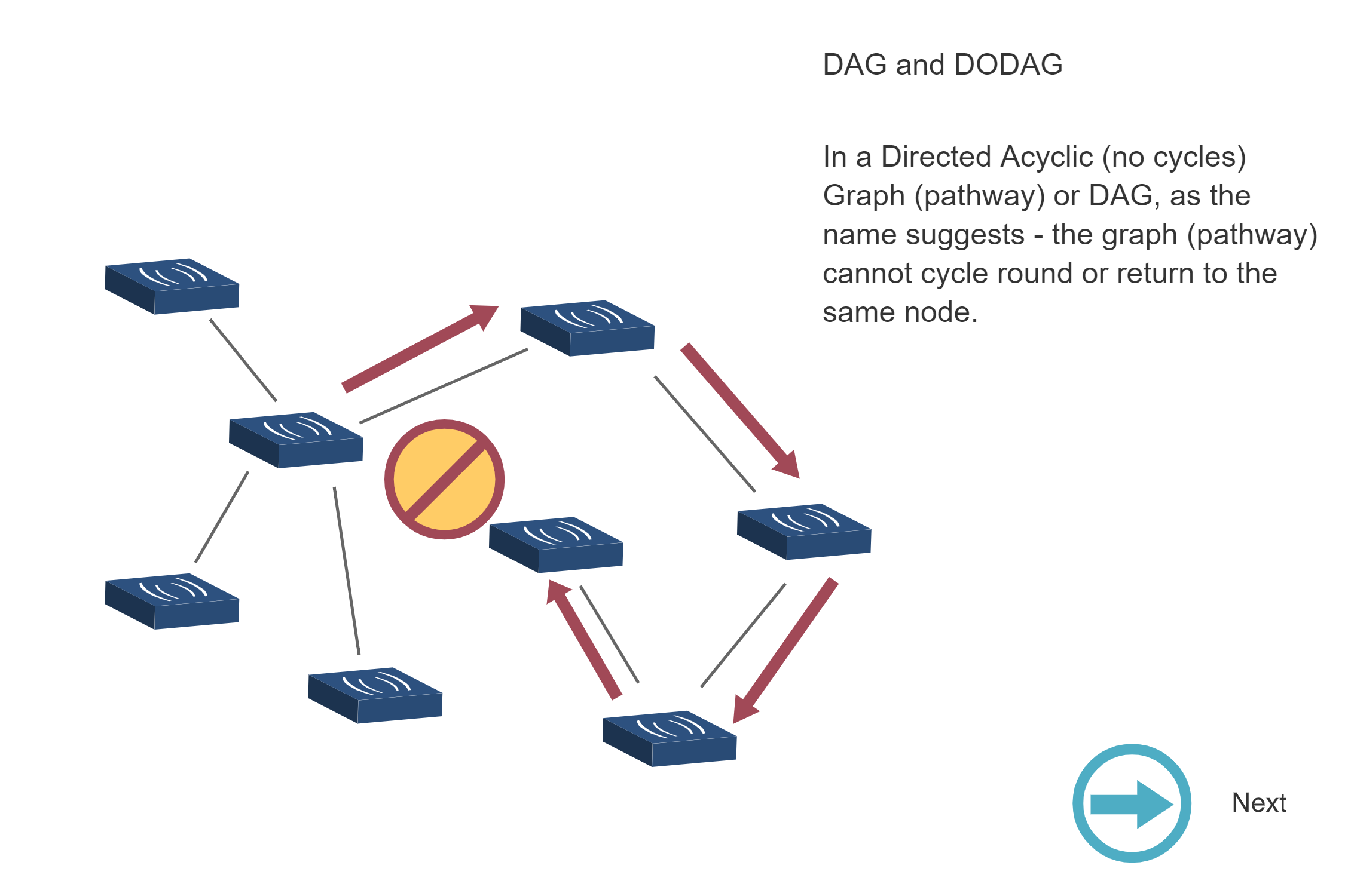
DAG and DODAG Structures (Source Figure)

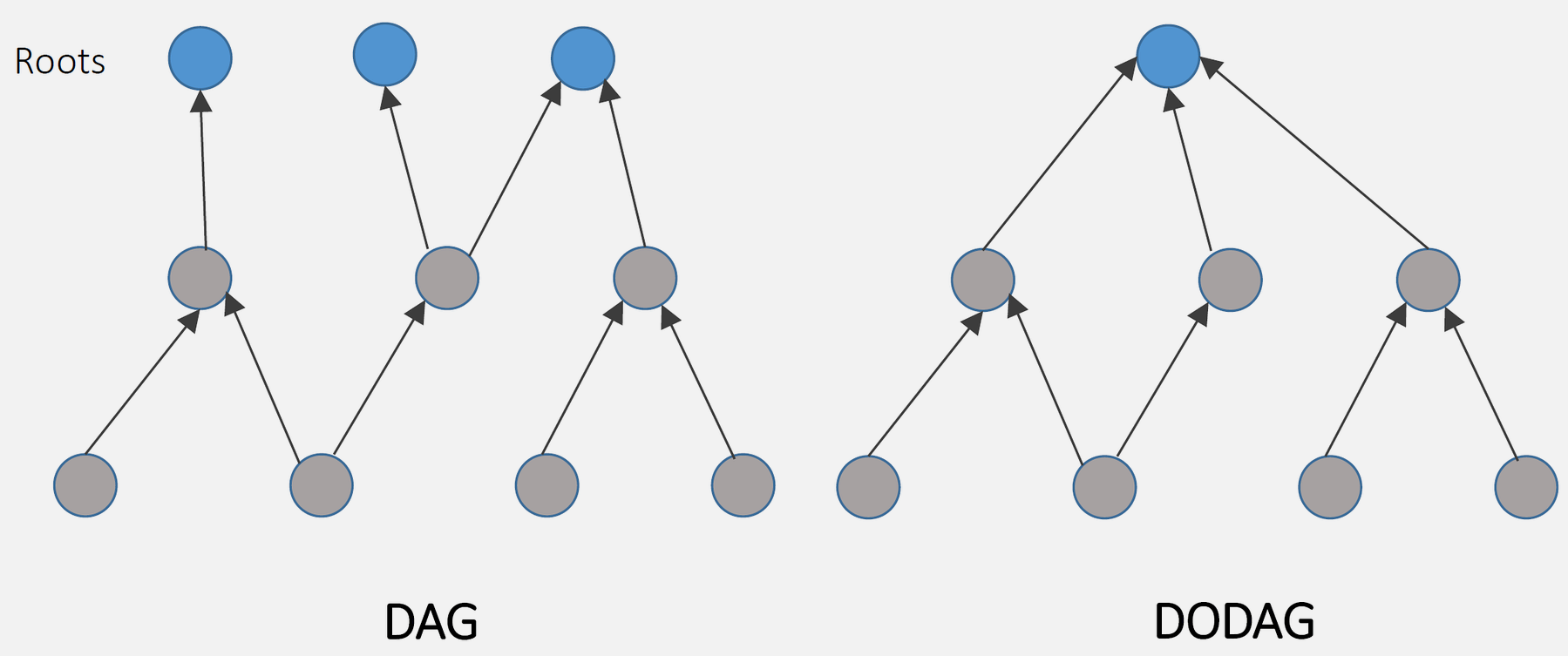
Original textbook figure showing the difference between a general Directed Acyclic Graph (DAG) with multiple roots and a DODAG (Destination-Oriented DAG) with a single root destination, illustrating how RPL creates tree-like structures for efficient IoT routing — DAG and DODAG comparison from original source

Source: CP IoT System Design Guide, Chapter 4 - Routing

RPL DAG and DODAG Formation Sequence

Step 1 of DODAG formation showing initial network state before RPL routing begins, with nodes scattered and no parent relationships established — RPL DAG and DODAG formation step 1

Step 2 of DODAG formation showing nodes beginning to receive DIO messages from the root and establishing initial parent selections — RPL DAG and DODAG formation step 2

Step 3 of DODAG formation showing complete tree structure with all nodes having selected preferred parents and routes to the root — RPL DAG and DODAG formation step 3

Source: CP IoT System Design Guide, Chapter 4 - Routing

RPL RANK Calculation Visualization

Complete visualization of RPL RANK values across a network showing how rank increases with distance from root, with root at rank 0 and leaf nodes at highest rank values — RPL Rank calculation overview

Step 1 of rank calculation showing root advertising rank 0 to immediate neighbors via DIO messages — RPL Rank step 1

Step 2 of rank calculation showing second-tier nodes calculating their rank based on parent rank plus link cost metric — RPL Rank step 2

Step 3 of rank calculation showing further propagation of rank values to deeper nodes in the network topology — RPL Rank step 3

Step 4 showing complete rank assignment across all nodes in the DODAG with final routing paths established — RPL Rank step 4

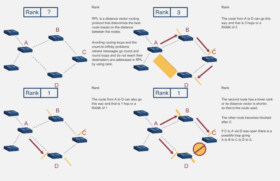
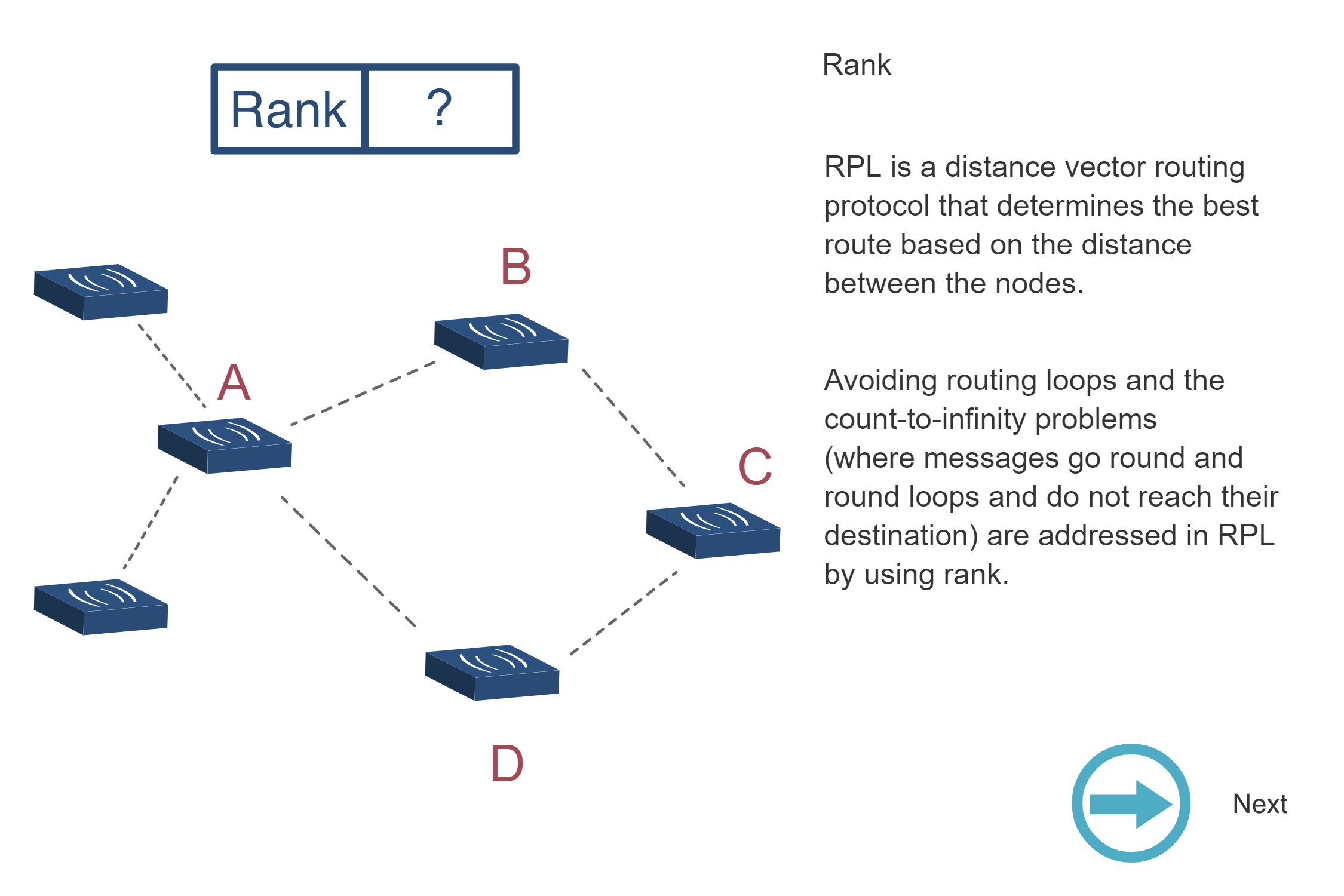
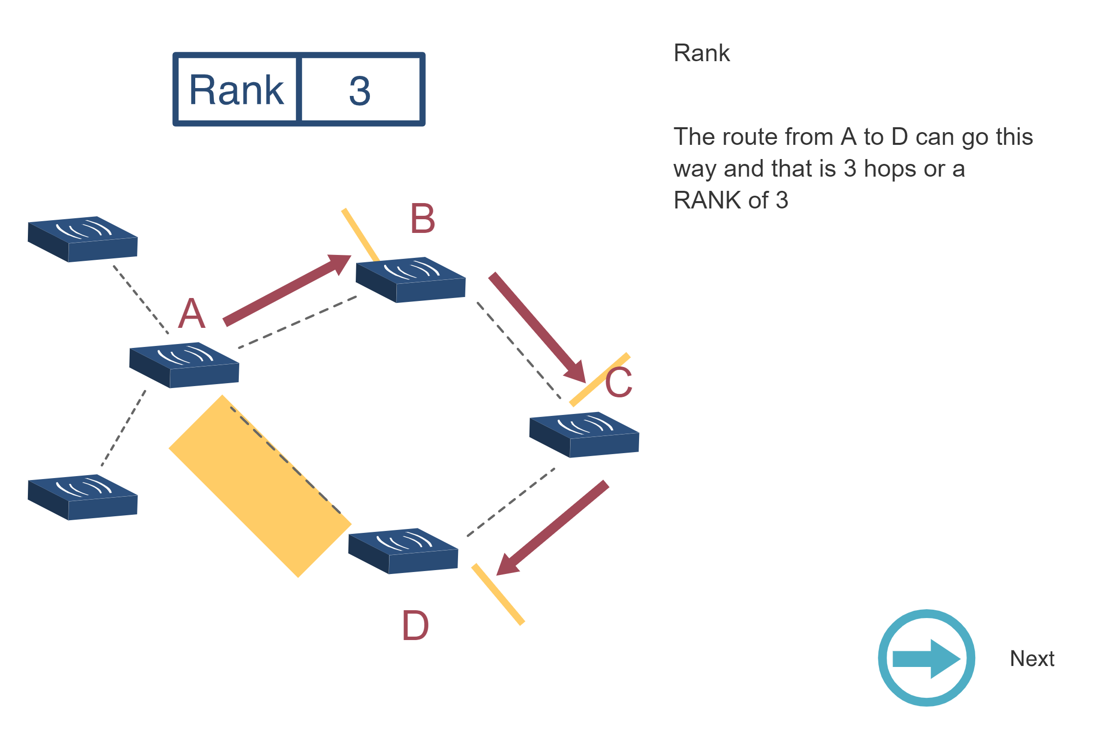
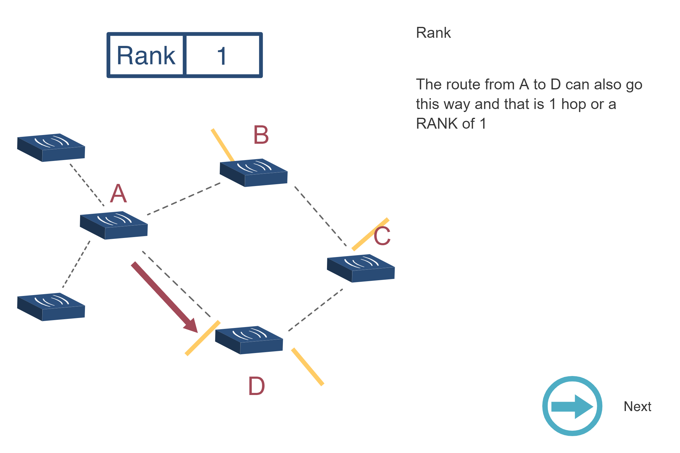
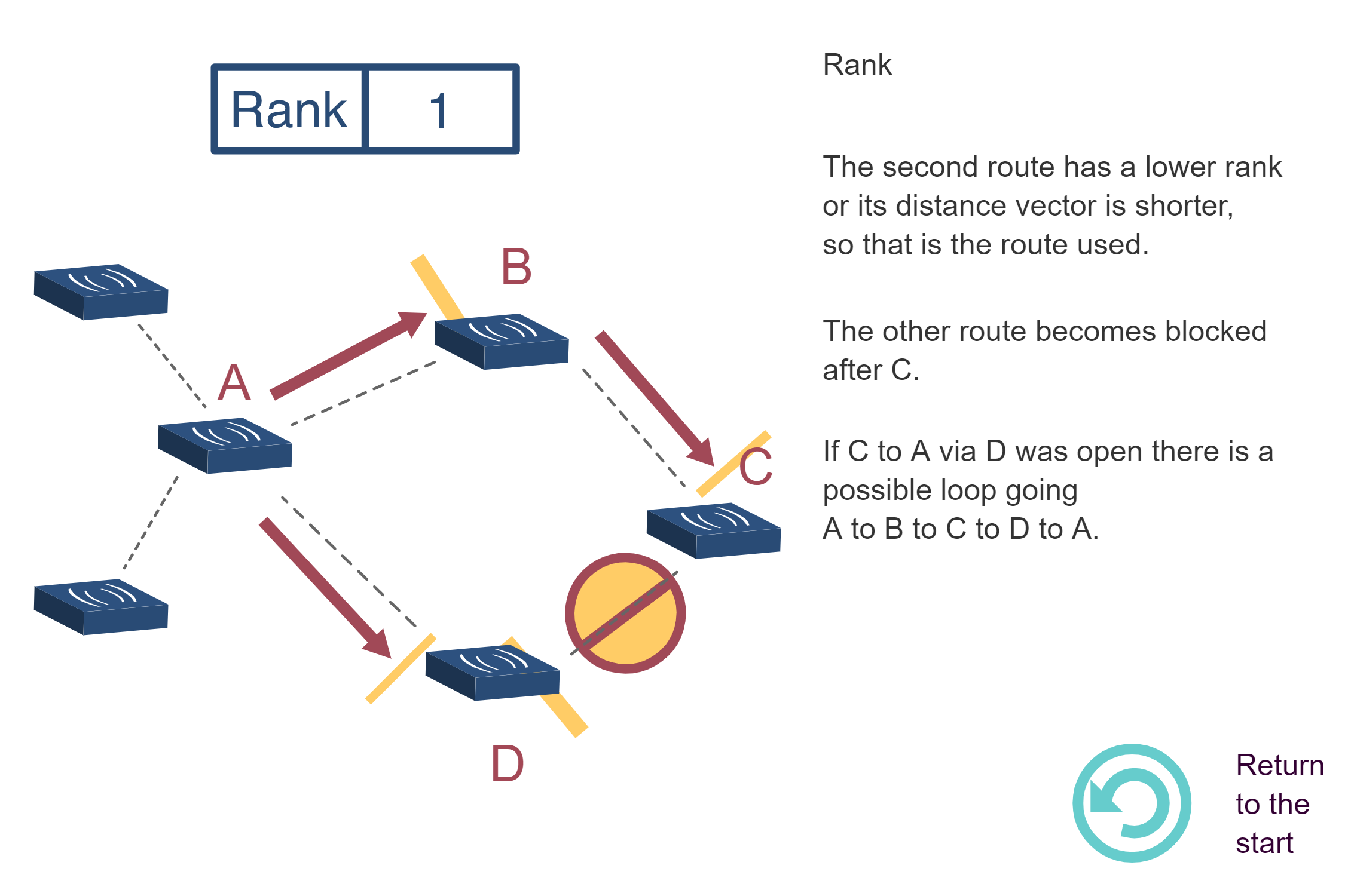
Source: CP IoT System Design Guide, Chapter 4 - Routing

Building a DODAG - Step-by-Step Process

Complete step-by-step visualization showing how a DODAG is constructed from initial state through final tree structure — Building a DODAG - Complete overview

DODAG building step 1: Root node initiates DODAG by sending first DIO message — Building a DODAG step 1

DODAG building step 2: Neighbors receive DIO, calculate rank, select root as parent — Building a DODAG step 2

DODAG building step 3: Second-tier nodes forward DIO messages to their neighbors — Building a DODAG step 3

DODAG building step 4: More nodes join DODAG, tree structure expands — Building a DODAG step 4

DODAG building step 5: Edge nodes receive DIO and select parents — Building a DODAG step 5

DODAG building step 6: Complete DODAG formed with all nodes having routes to root — Building a DODAG step 6

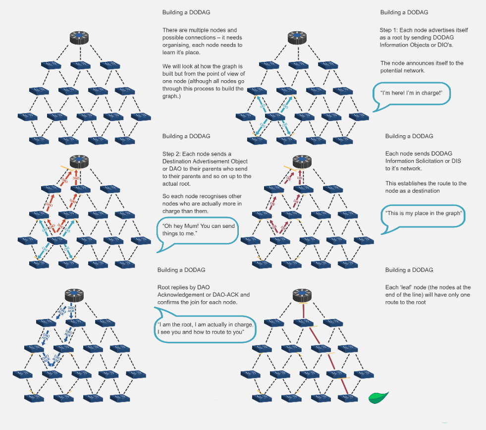
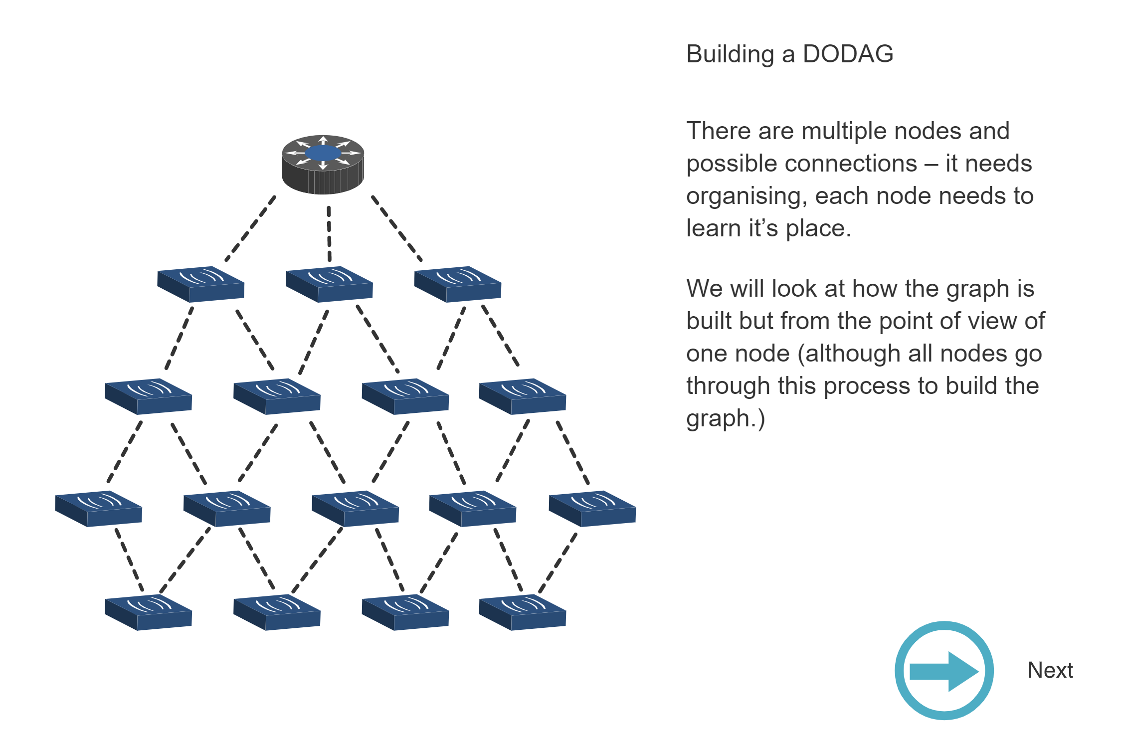
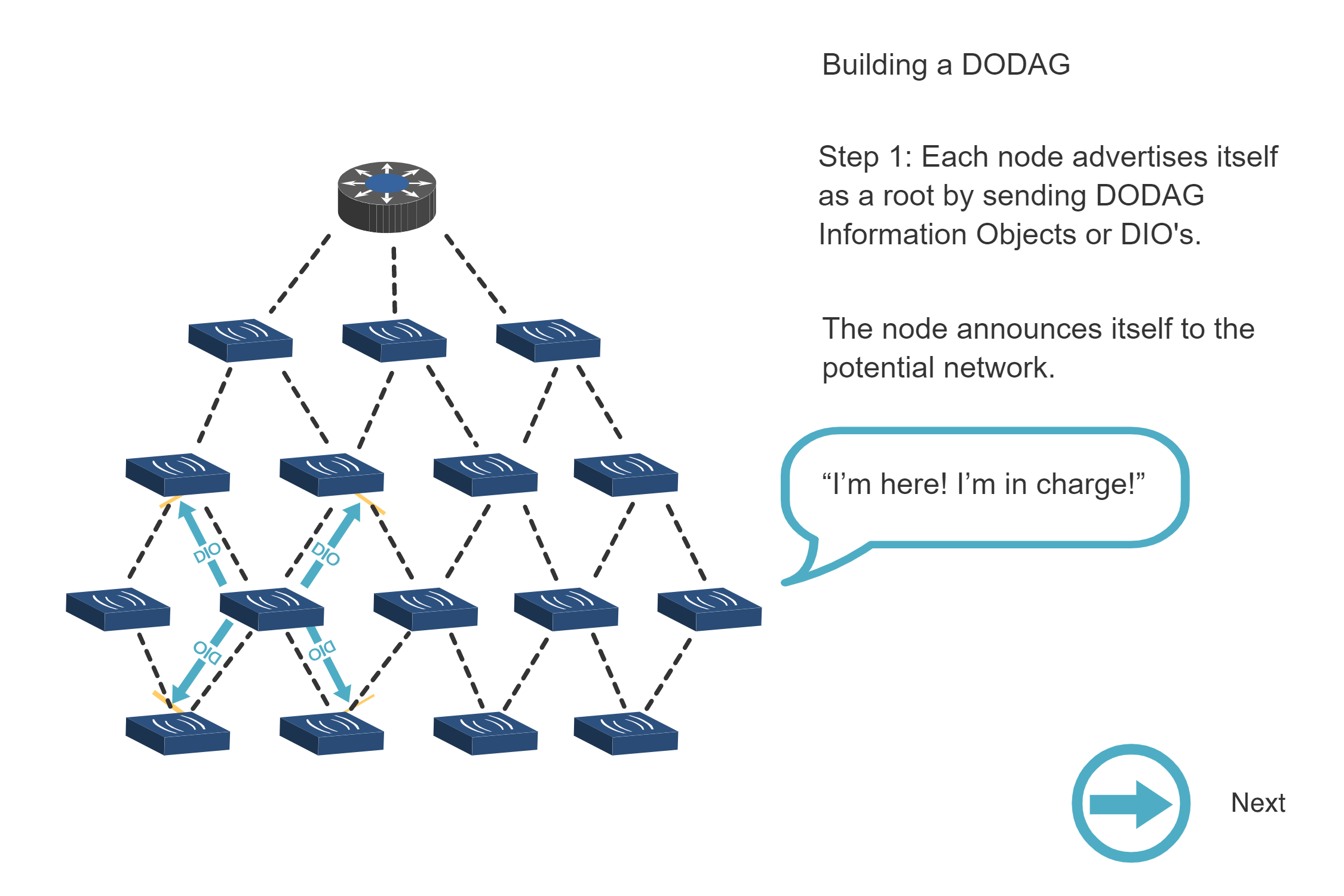
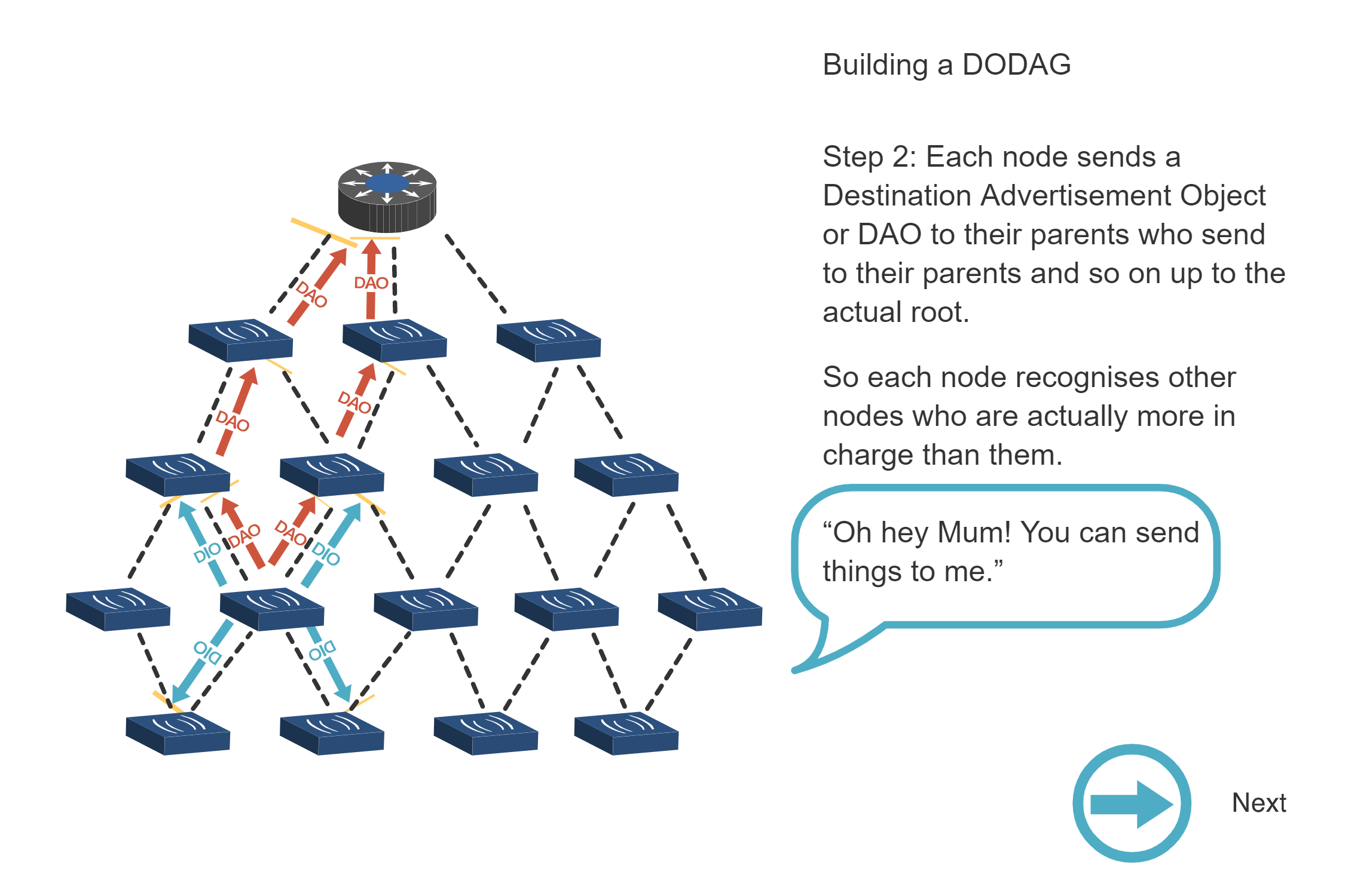
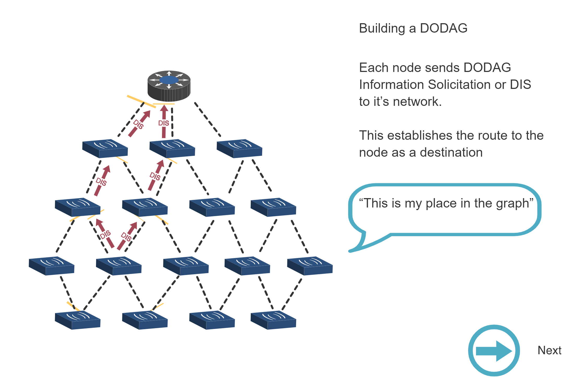
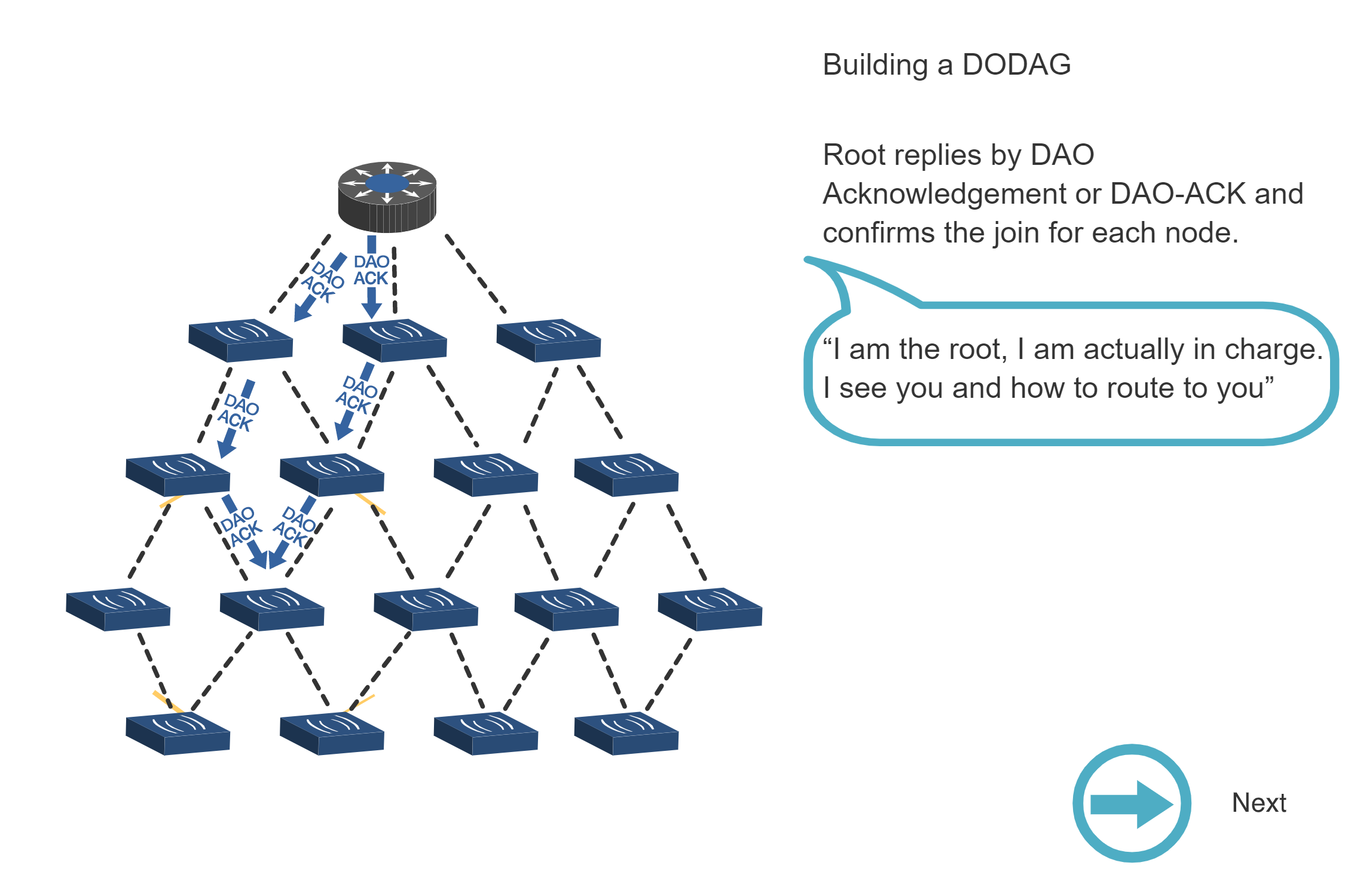
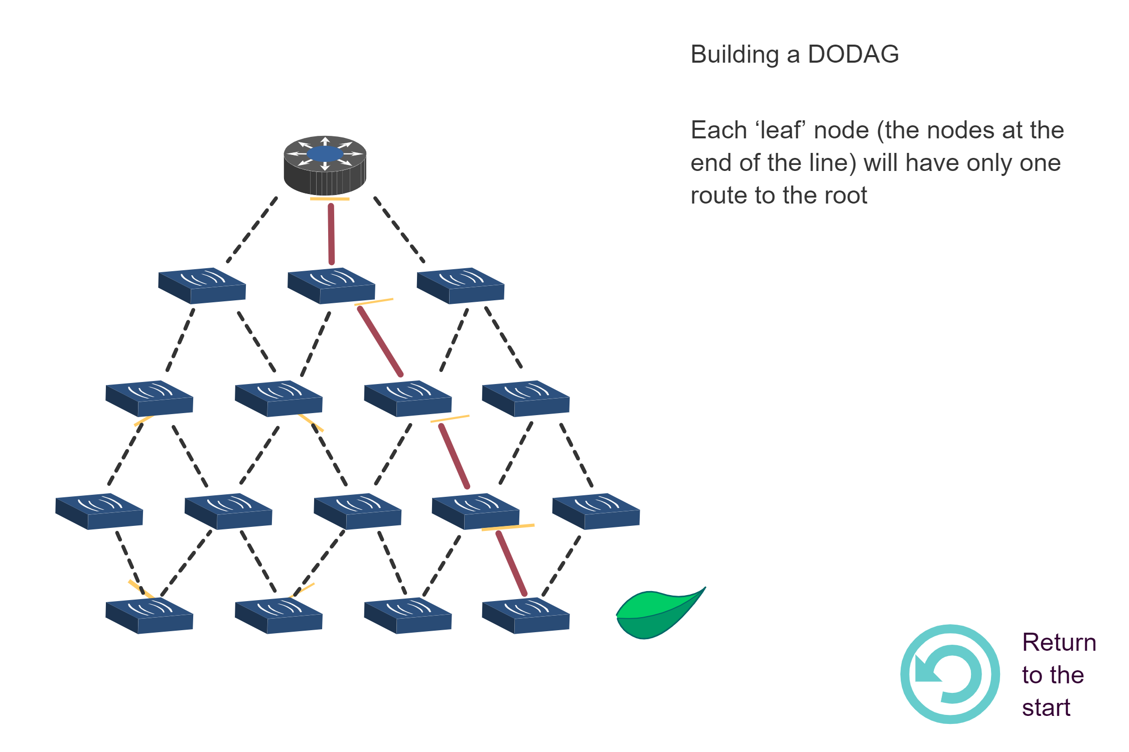
Source: CP IoT System Design Guide, Chapter 4 - Routing

Interactive: RPL DODAG Builder

Build and visualize an RPL DODAG (Destination Oriented Directed Acyclic Graph) interactively. Watch how nodes join the network, calculate their RANK based on different objective functions, and see DIO messages propagate through the tree.

Instructions:

Click “Add Node” to add new nodes to the network
Select different Objective Functions to see how RANK calculation changes
Watch how each node selects its parent based on the objective function
Observe the DIO propagation from root outward
Use “Reset Network” to start fresh

Show code

viewof objectiveFunction = Inputs.select(
  ["hop_count", "etx", "energy"],
  {
    value: "hop_count",
    label: "Objective Function",
    format: x => x === "hop_count" ? "Hop Count (OF0 - simple)" :
                 x === "etx" ? "ETX (Expected Transmission Count)" :
                 "Energy (minimize power consumption)"
  }
)

Show code

initialRoot = [{id: 0, name: "ROOT", x: 400, y: 50, rank: 0, parent: null, isRoot: true, etx: 1.0, energy: 100}]

mutable dodagNodes = initialRoot

mutable nodeCounter = 1

mutable messageLog = ["Network initialized. ROOT node created at RANK 0."]

Show code

function createNode(nodes, of, counter) {
  const layer = Math.floor(nodes.length / 3) + 1
  const nodesInLayer = nodes.filter(n => Math.floor(n.rank / 256) === layer - 1).length
  const xOffset = (nodesInLayer % 3 - 1) * 150
  const newX = Math.max(50, Math.min(750, 400 + xOffset + (Math.random() - 0.5) * 80))
  const newY = Math.max(100, Math.min(450, 50 + layer * 100 + (Math.random() - 0.5) * 30))

  const etxVal = 1.0 + Math.random() * 2.0
  const energyCost = 50 + Math.random() * 100

  let bestParent = null
  let bestCost = Infinity

  for (const p of nodes.filter(n => n.rank < 65535)) {
    const dist = Math.sqrt(Math.pow(newX - p.x, 2) + Math.pow(newY - p.y, 2))
    if (dist > 250) continue

    let cost = p.rank + 256
    if (of === "etx") cost = p.rank + Math.floor(etxVal * 256)
    else if (of === "energy") cost = p.rank + Math.floor(energyCost * 2)

    if (cost < bestCost) {
      bestCost = cost
      bestParent = p
    }
  }

  if (!bestParent) {
    bestParent = nodes.reduce((a, b) => {
      const distA = Math.sqrt(Math.pow(newX - a.x, 2) + Math.pow(newY - a.y, 2))
      const distB = Math.sqrt(Math.pow(newX - b.x, 2) + Math.pow(newY - b.y, 2))
      return distA < distB ? a : b
    })
    bestCost = bestParent.rank + 256
    if (of === "etx") bestCost = bestParent.rank + Math.floor(etxVal * 256)
    else if (of === "energy") bestCost = bestParent.rank + Math.floor(energyCost * 2)
  }

  return {
    id: counter,
    name: "Node " + String.fromCharCode(65 + counter - 1),
    x: newX,
    y: newY,
    rank: bestCost,
    parent: bestParent.id,
    parentName: bestParent.name,
    isRoot: false,
    etx: etxVal,
    energy: energyCost
  }
}

Show code

viewof addNodeBtn = Inputs.button("Add Node", {
  reduce: () => {
    if (dodagNodes.length >= 15) {
      mutable messageLog = [...messageLog.slice(-9), "Maximum 15 nodes reached. Reset to add more."]
      return
    }
    const newNode = createNode(dodagNodes, objectiveFunction, nodeCounter)
    mutable dodagNodes = [...dodagNodes, newNode]
    mutable nodeCounter = nodeCounter + 1
    const ofLabel = objectiveFunction === "hop_count" ? "Hop Count" :
                    objectiveFunction === "etx" ? "ETX" : "Energy"
    mutable messageLog = [...messageLog.slice(-9),
      "DIO received: " + newNode.name + " joined. Parent: " + newNode.parentName + ", RANK: " + newNode.rank + " (" + ofLabel + ")"
    ]
  }
})

viewof resetBtn = Inputs.button("Reset Network", {
  reduce: () => {
    mutable dodagNodes = initialRoot
    mutable nodeCounter = 1
    mutable messageLog = ["Network reset. ROOT node created at RANK 0."]
  }
})

Show code

dodagVisualization = {
  const width = 800
  const height = 500

  const svg = d3.create("svg")
    .attr("viewBox", [0, 0, width, height])
    .attr("width", "100%")
    .attr("height", height)
    .style("background", "#f8f9fa")
    .style("border-radius", "8px")
    .style("border", "1px solid #dee2e6")

  svg.append("text")
    .attr("x", width / 2)
    .attr("y", 25)
    .attr("text-anchor", "middle")
    .attr("font-size", "14px")
    .attr("font-weight", "bold")
    .attr("fill", "#2C3E50")
    .text("RPL DODAG Visualization")

  const edges = dodagNodes.filter(n => n.parent !== null)

  svg.selectAll("line.edge")
    .data(edges)
    .join("line")
    .attr("class", "edge")
    .attr("x1", d => dodagNodes.find(n => n.id === d.parent).x)
    .attr("y1", d => dodagNodes.find(n => n.id === d.parent).y)
    .attr("x2", d => d.x)
    .attr("y2", d => d.y)
    .attr("stroke", "#16A085")
    .attr("stroke-width", 2)
    .attr("stroke-dasharray", d => d.id === dodagNodes[dodagNodes.length - 1].id && dodagNodes.length > 1 ? "5,5" : "none")
    .attr("opacity", d => d.id === dodagNodes[dodagNodes.length - 1].id && dodagNodes.length > 1 ? 0.7 : 1)

  if (dodagNodes.length > 1) {
    const newest = dodagNodes[dodagNodes.length - 1]
    const parent = dodagNodes.find(n => n.id === newest.parent)
    if (parent) {
      const pulse = svg.append("circle")
        .attr("cx", parent.x)
        .attr("cy", parent.y)
        .attr("r", 5)
        .attr("fill", "#E67E22")
        .attr("opacity", 0.8)
      pulse.append("animate")
        .attr("attributeName", "r")
        .attr("from", 5)
        .attr("to", 30)
        .attr("dur", "1s")
        .attr("repeatCount", "3")
      pulse.append("animate")
        .attr("attributeName", "opacity")
        .attr("from", 0.8)
        .attr("to", 0)
        .attr("dur", "1s")
        .attr("repeatCount", "3")
    }
  }

  const nodeGroups = svg.selectAll("g.node")
    .data(dodagNodes)
    .join("g")
    .attr("class", "node")
    .attr("transform", d => "translate(" + d.x + ", " + d.y + ")")

  nodeGroups.append("circle")
    .attr("r", d => d.isRoot ? 25 : 20)
    .attr("fill", d => d.isRoot ? "#2C3E50" :
      d.id === dodagNodes[dodagNodes.length - 1].id && dodagNodes.length > 1 ? "#E67E22" : "#16A085")
    .attr("stroke", d => d.isRoot ? "#16A085" : "#2C3E50")
    .attr("stroke-width", d => d.isRoot ? 3 : 2)

  nodeGroups.append("text")
    .attr("text-anchor", "middle")
    .attr("dy", -30)
    .attr("font-size", "12px")
    .attr("font-weight", "bold")
    .attr("fill", "#2C3E50")
    .text(d => d.name)

  nodeGroups.append("text")
    .attr("text-anchor", "middle")
    .attr("dy", 5)
    .attr("font-size", "10px")
    .attr("fill", "white")
    .attr("font-weight", "bold")
    .text(d => d.rank)

  nodeGroups.append("text")
    .attr("text-anchor", "middle")
    .attr("dy", 35)
    .attr("font-size", "9px")
    .attr("fill", "#7F8C8D")
    .text(d => "RANK: " + d.rank)

  const legend = svg.append("g")
    .attr("transform", "translate(20, " + (height - 100) + ")")

  legend.append("rect")
    .attr("width", 180)
    .attr("height", 90)
    .attr("fill", "white")
    .attr("stroke", "#dee2e6")
    .attr("rx", 4)

  legend.append("text").attr("x", 10).attr("y", 18)
    .attr("font-size", "11px").attr("font-weight", "bold").attr("fill", "#2C3E50")
    .text("Legend:")

  legend.append("circle").attr("cx", 20).attr("cy", 38).attr("r", 8)
    .attr("fill", "#2C3E50").attr("stroke", "#16A085").attr("stroke-width", 2)
  legend.append("text").attr("x", 35).attr("y", 42)
    .attr("font-size", "10px").attr("fill", "#2C3E50").text("ROOT (RANK 0)")

  legend.append("circle").attr("cx", 20).attr("cy", 58).attr("r", 8).attr("fill", "#16A085")
  legend.append("text").attr("x", 35).attr("y", 62)
    .attr("font-size", "10px").attr("fill", "#2C3E50").text("Joined Node")

  legend.append("circle").attr("cx", 20).attr("cy", 78).attr("r", 8).attr("fill", "#E67E22")
  legend.append("text").attr("x", 35).attr("y", 82)
    .attr("font-size", "10px").attr("fill", "#2C3E50").text("Just Joined (DIO pulse)")

  const stats = svg.append("g")
    .attr("transform", "translate(" + (width - 200) + ", " + (height - 100) + ")")

  stats.append("rect").attr("width", 180).attr("height", 90)
    .attr("fill", "white").attr("stroke", "#dee2e6").attr("rx", 4)

  stats.append("text").attr("x", 10).attr("y", 18)
    .attr("font-size", "11px").attr("font-weight", "bold").attr("fill", "#2C3E50")
    .text("Network Stats:")

  stats.append("text").attr("x", 10).attr("y", 38)
    .attr("font-size", "10px").attr("fill", "#2C3E50")
    .text("Nodes: " + dodagNodes.length)

  const maxRank = Math.max(...dodagNodes.map(n => n.rank))
  const maxDepth = Math.ceil(maxRank / 256)

  stats.append("text").attr("x", 10).attr("y", 54)
    .attr("font-size", "10px").attr("fill", "#2C3E50")
    .text("Max RANK: " + maxRank)

  stats.append("text").attr("x", 10).attr("y", 70)
    .attr("font-size", "10px").attr("fill", "#2C3E50")
    .text("Est. Depth: ~" + maxDepth + " hops")

  const ofName = objectiveFunction === "hop_count" ? "Hop Count" :
                 objectiveFunction === "etx" ? "ETX" : "Energy"
  stats.append("text").attr("x", 10).attr("y", 86)
    .attr("font-size", "10px").attr("fill", "#2C3E50")
    .text("OF: " + ofName)

  return svg.node()
}

Show code

messageLogDisplay = html`<div style="background: #2C3E50; color: #16A085; padding: 12px; border-radius: 4px; font-family: monospace; font-size: 11px; max-height: 150px; overflow-y: auto; margin-top: 10px;">
  <div style="color: #E67E22; font-weight: bold; margin-bottom: 8px;">DIO/DAO Message Log (Trickle Timer Active):</div>
  ${messageLog.map(msg => html`<div style="margin: 2px 0; color: ${msg.includes('DIO') ? '#16A085' : msg.includes('reset') ? '#E67E22' : '#fff'};">-> ${msg}</div>`)}
</div>`

Show code

trickleInfo = html`<div style="background: #f8f9fa; border: 1px solid #dee2e6; border-radius: 4px; padding: 12px; margin-top: 10px;">
  <div style="font-weight: bold; color: #2C3E50; margin-bottom: 8px;">Trickle Timer Concept:</div>
  <div style="font-size: 12px; color: #495057; line-height: 1.5;">
    <p>In real RPL networks, the <strong>Trickle Timer</strong> controls DIO message frequency:</p>
    <ul style="margin: 8px 0;">
      <li><strong>Stable network</strong>: DIOs sent infrequently (minutes) to save energy</li>
      <li><strong>Network change</strong>: Timer resets, DIOs sent frequently (seconds) for fast convergence</li>
      <li><strong>Suppression</strong>: If neighbors already sent consistent DIOs, skip own transmission</li>
    </ul>
    <p style="color: #16A085;"><strong>Current simulation</strong>: Each "Add Node" simulates receiving a DIO and joining the DODAG. The orange pulse shows DIO propagation from the parent.</p>
  </div>
</div>`

Objective Function Details:

Function	RANK Calculation	Best For
Hop Count (OF0)	Parent RANK + 256 per hop	Simple networks, equal link quality
ETX	Parent RANK + (ETX x 256)	Lossy networks, reliability focus
Energy	Parent RANK + (Energy x 2)	Battery-powered, lifetime optimization

Try This:

Add 5-6 nodes and observe the tree structure
Switch objective functions and reset - notice how the same nodes may select different parents
Watch the orange DIO pulse showing message propagation
Note how RANK increases as you move away from ROOT

701.11 Summary

This chapter covered the Trickle algorithm and RPL routing modes:

Trickle Algorithm: Adaptive control message timing that achieves 99.7% reduction in DIO overhead through exponential backoff and instant reset on inconsistency
Three Scenarios: Stable network (doubling interval), inconsistency (reset interval), insufficient redundancy (broadcast)
Storing Mode: Distributed routing tables enable optimal paths but require more memory per node
Non-Storing Mode: Centralized routing at root minimizes node memory but routes through root
Traffic Patterns: Many-to-one (upward), one-to-many (downward), and point-to-point routing
Common Pitfalls: Wrong mode selection, aggressive Trickle settings, single root without redundancy

701.12 What’s Next

Continue to RPL Labs and Quiz to apply your understanding through hands-on network design exercises and test your knowledge with comprehensive quiz questions.