715 RPL DODAG Visual Construction Guide
715.1 Learning Objectives
After completing this chapter, you will be able to:
- Visualize the 5-phase DODAG construction algorithm
- Understand the temporal dynamics of DODAG formation (7-step process)
- Distinguish between DAG and DODAG structures
- Identify the timing of each formation phase in real networks
715.2 DODAG Construction: Visual Algorithm
This condensed visual sequence shows the 5 key phases of DODAG construction. Each diagram focuses on one step, making the algorithm easy to understand and remember.
715.2.1 Step 1: Root Initialization

{fig-alt=“Step 1 of DODAG construction algorithm showing Root node at Rank 0 (orange) broadcasting DIO messages to three unknown nodes (gray question marks) that have not yet joined the network”}
What happens: Root broadcasts DIO containing Rank=0, DODAG ID, and objective function. Neighboring nodes receive but haven’t processed yet.
715.2.2 Step 2: First-Hop Join
{fig-alt=“Step 2 of DODAG construction showing first-hop nodes A, B, and C (green) joining the network with calculated Rank values of 256, 256, and 384 respectively, connected to the Root node”}
What happens: Nodes hear DIO, calculate Rank = Parent_Rank + Link_Cost, and select root as parent. Node C has higher Rank (384) due to poorer link quality.
715.2.3 Step 3: Multi-Hop Expansion
{fig-alt=“Step 3 showing multi-hop expansion with nodes D and E (dark blue) joining at Rank 512 through their parents A and B, forming a two-level tree structure below the root”}
What happens: First-hop nodes broadcast their own DIO messages. Second-hop nodes (D, E) join with Rank = 256 + 256 = 512. Process ripples outward hop-by-hop until all nodes join the DODAG.
715.2.4 Step 4: DAO Propagation
{fig-alt=“Step 4 showing DAO message propagation flowing upward from leaf nodes D and E through intermediate nodes A and B toward the Root, building downward routing tables for optional two-way communication”}
What happens: Nodes send DAO (Destination Advertisement Object) messages toward the root to establish downward routes. This enables the root (and intermediate nodes in storing mode) to send data to specific nodes.
715.2.5 Step 5: Steady State
{fig-alt=“Step 5 showing complete DODAG in steady state with all nodes joined, parent relationships established, and downward routes available at the root for bidirectional communication”}
What happens: DODAG complete! Trickle algorithm now maintains consistency with minimal overhead—DIO messages become rare when network is stable. If a node fails, neighbors detect it and repair locally.
| Step | Action | Messages | Result |
|---|---|---|---|
| 1 | Root init | DIO broadcast | DODAG announced |
| 2 | First-hop join | DIO received | Nodes calculate Rank, select parent |
| 3 | Multi-hop expand | DIO ripple outward | All nodes join progressively |
| 4 | Downward routes | DAO toward root | Root learns paths to all nodes |
| 5 | Steady state | Trickle-controlled DIO | Minimal overhead, self-healing |
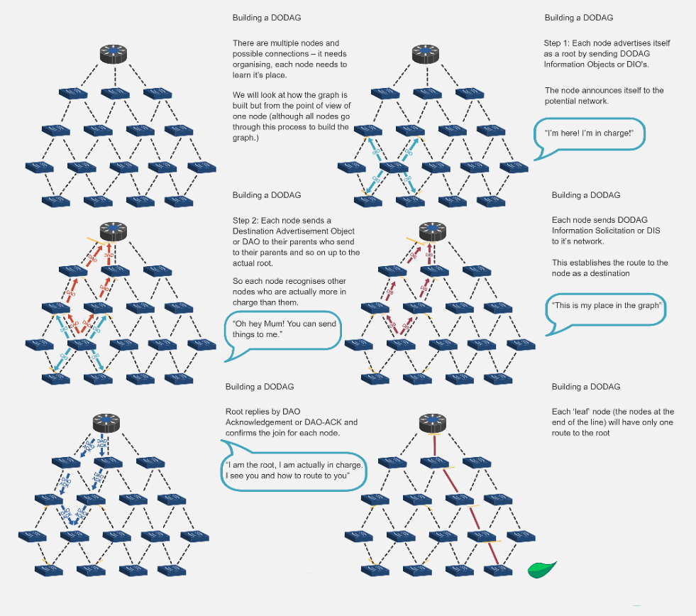
715.3 DODAG Formation: Step-by-Step Visual Guide
The following sequence shows how a DODAG forms step-by-step in a real network. This progressive visualization helps you understand the temporal dynamics of RPL—not just the final topology, but how nodes discover each other and build the routing structure over time.
Understanding how RPL networks self-organize from chaos to hierarchy is crucial for troubleshooting and optimization. This 7-step visual progression shows the complete DODAG construction process with real timing information.
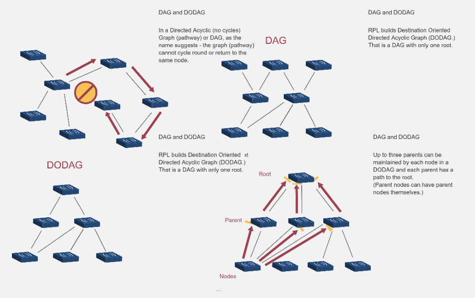
715.3.1 Understanding DAG vs DODAG First
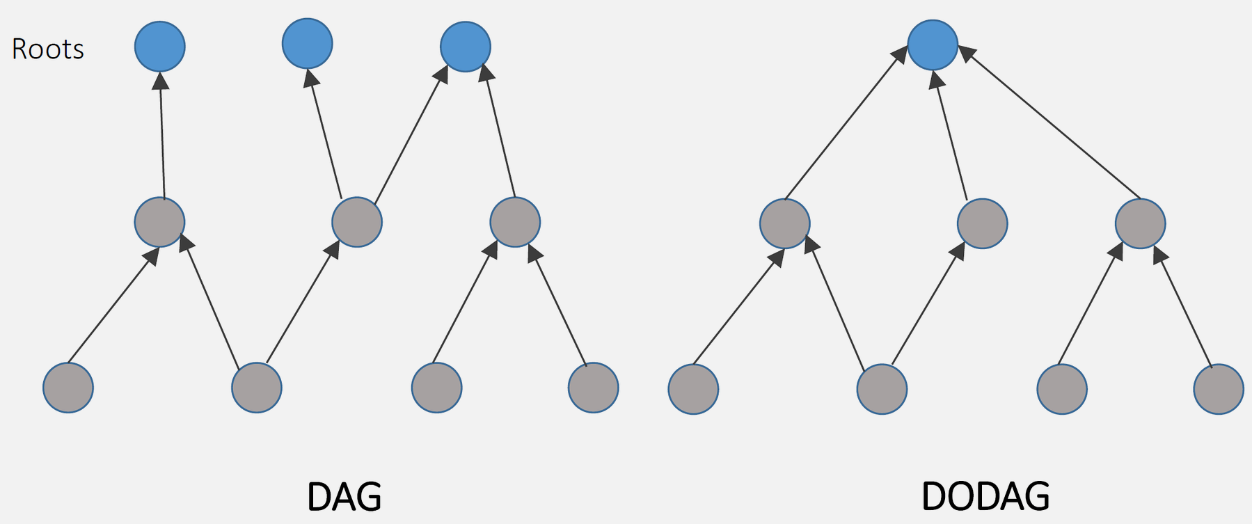
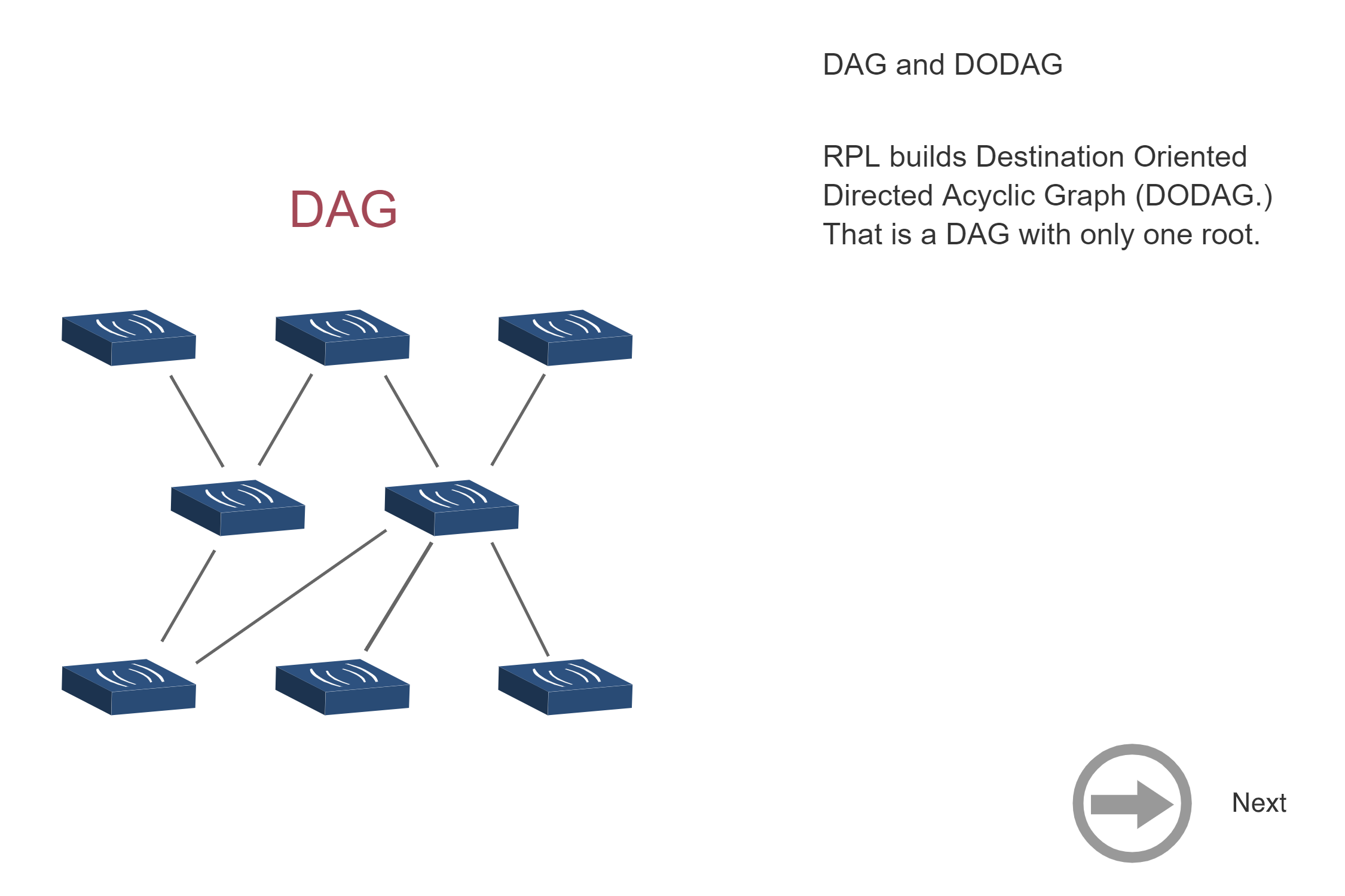

Key Difference: A DAG can have multiple independent trees with separate roots. A DODAG has exactly one root (the gateway/border router) where all paths converge. This single-destination orientation is perfect for IoT’s many-to-one traffic pattern (sensors -> cloud).
715.3.2 The 7-Step DODAG Formation Process
This visual sequence shows how RPL transforms unorganized nodes into a self-healing hierarchical network. Pay attention to the timing and message flow at each step—understanding the process is more important than memorizing the final topology.
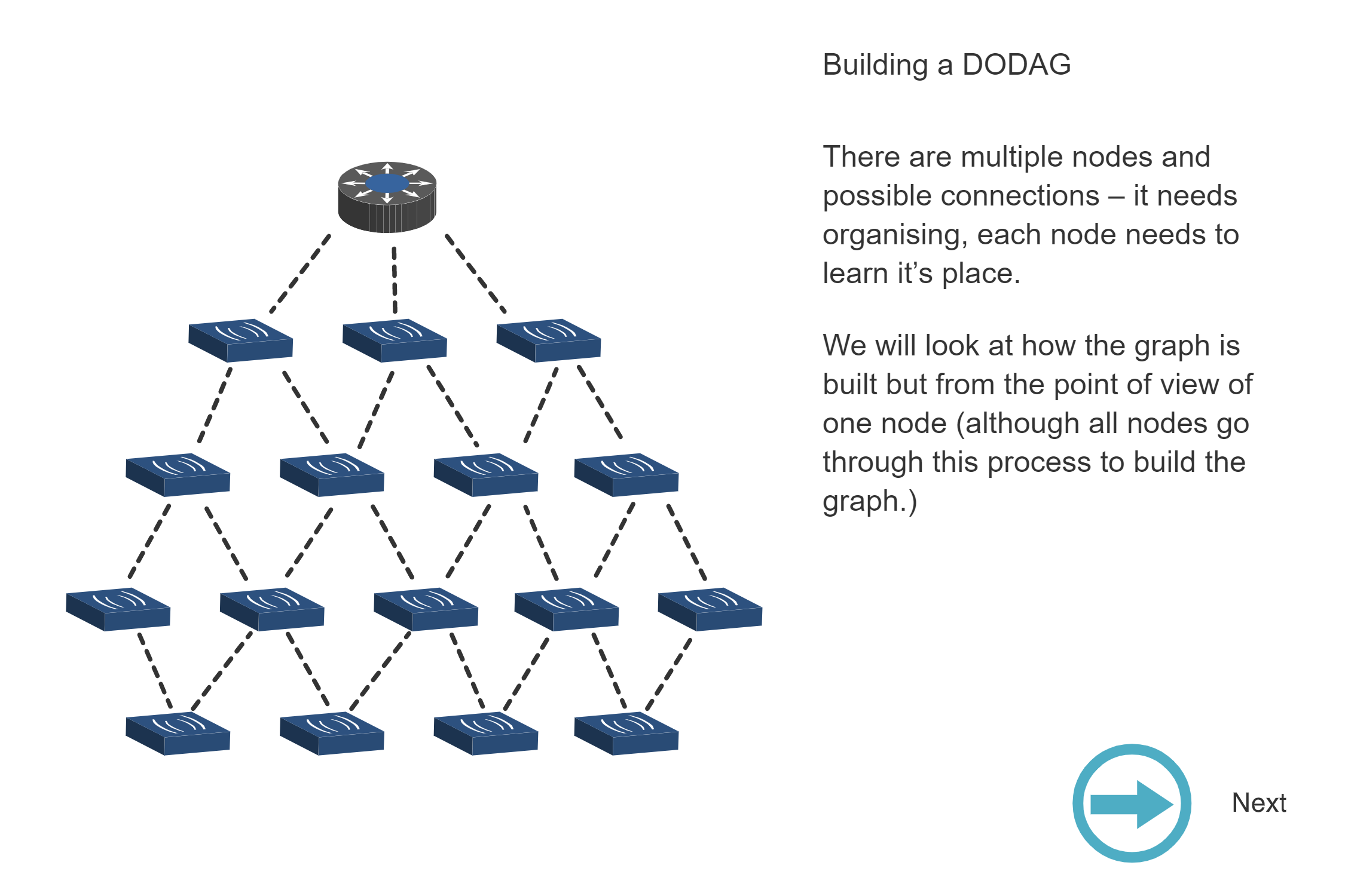
715.3.2.1 Step 1: Initial State - Unorganized Network
Network State: - One designated root (border router/gateway) at top - Multiple sensor nodes powered on and ready - All connections are potential (dotted lines = physical radio range) - Nodes don’t know their parents or RANK values yet - Network needs to self-organize from chaos to hierarchy
What nodes know: Their own address, radio is on, listening for RPL messages
What nodes don’t know: Who is the root, what DODAG to join, which neighbor to use as parent
Real-world timing: This is the state at t=0 seconds when you power on a network
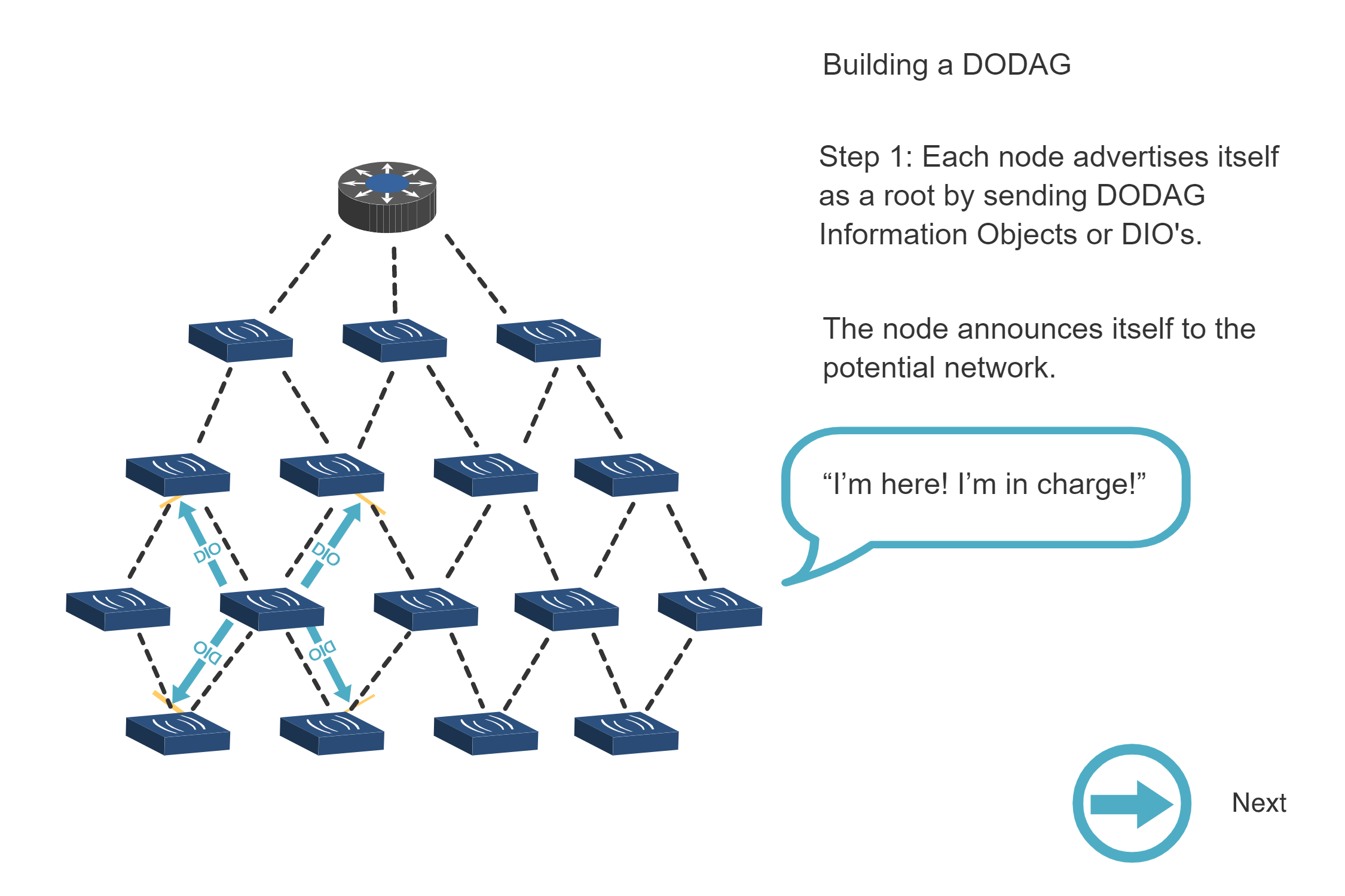
715.3.2.2 Step 2: Root Broadcasts DIO (t = 0-2 seconds)
Root Initiates DODAG (DIO Broadcast)
The root initiates DODAG construction by broadcasting DIO (DODAG Information Object) messages:
- Message content: “I am the root, RANK = 0, DODAG_ID = [IPv6 address], Objective Function = ETX”
- Who receives: All nodes within radio range of root (first-hop neighbors, shown in row 2)
- Propagation: Multicast to all neighbors (efficient broadcast using IPv6 multicast)
- RANK announced: Root advertises RANK = 0
- Analogy: Root announces “I’m here! I’m in charge!” to nearby nodes
First-hop nodes receive DIO: - Calculate their own RANK: RANK = 0 + rank_increase (typically 100-256) - Select root as their parent (best option available) - Store DODAG_ID and configuration
Real-world timing: DIO sent immediately on root startup (t=0-2s), then controlled by trickle timer
Key insight: Only nodes in radio range hear this first DIO. Network expands outward in a “ripple effect” as these nodes forward DIOs in later steps.
715.3.2.3 Step 3: First-Hop Nodes Join & Propagate (t = 2-5 seconds)
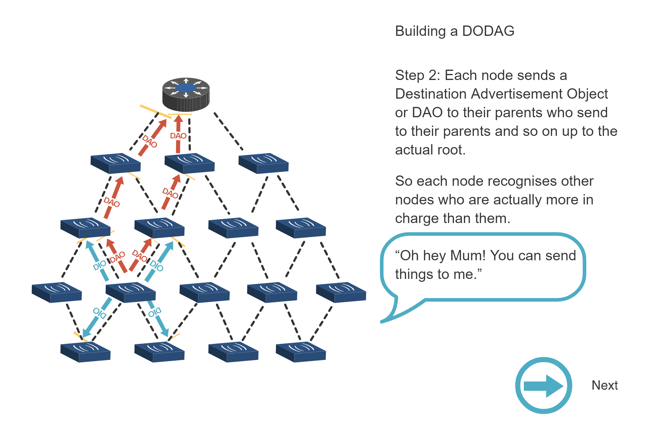
Nodes Join and Send DAO Messages Upward
First-hop nodes (row 2) now participate in DODAG:
- Nodes send DAO (Destination Advertisement Object) messages upward to root:
- Message content: “I am reachable via you, my address is [IPv6]”
- Direction: Child -> Parent (upward toward root)
- Purpose: Build downward routes so root can send commands/updates to specific nodes
- Storing mode: Root stores routing table entry: “Node X reachable via this interface”
- Nodes send own DIOs to their neighbors (row 3):
- Advertise their RANK (e.g., RANK = 256)
- Propagate DODAG information outward
- Enable row 3 nodes to join in next step
- Analogy: “Hey parent! You can send things to me” (DAO upward) + “Hey neighbors! Join this DODAG” (DIO outward)
Real-world timing: DAO sent 1-3 seconds after receiving DIO (in Storing mode)
Ripple effect: Network expands outward as each layer joins and forwards DIOs to the next layer
715.3.2.4 Step 4: DODAG Expands Outward (t = 5-10 seconds)
Deeper Nodes Request and Join
Nodes in rows 3 and 4 (farther from root) now join DODAG:
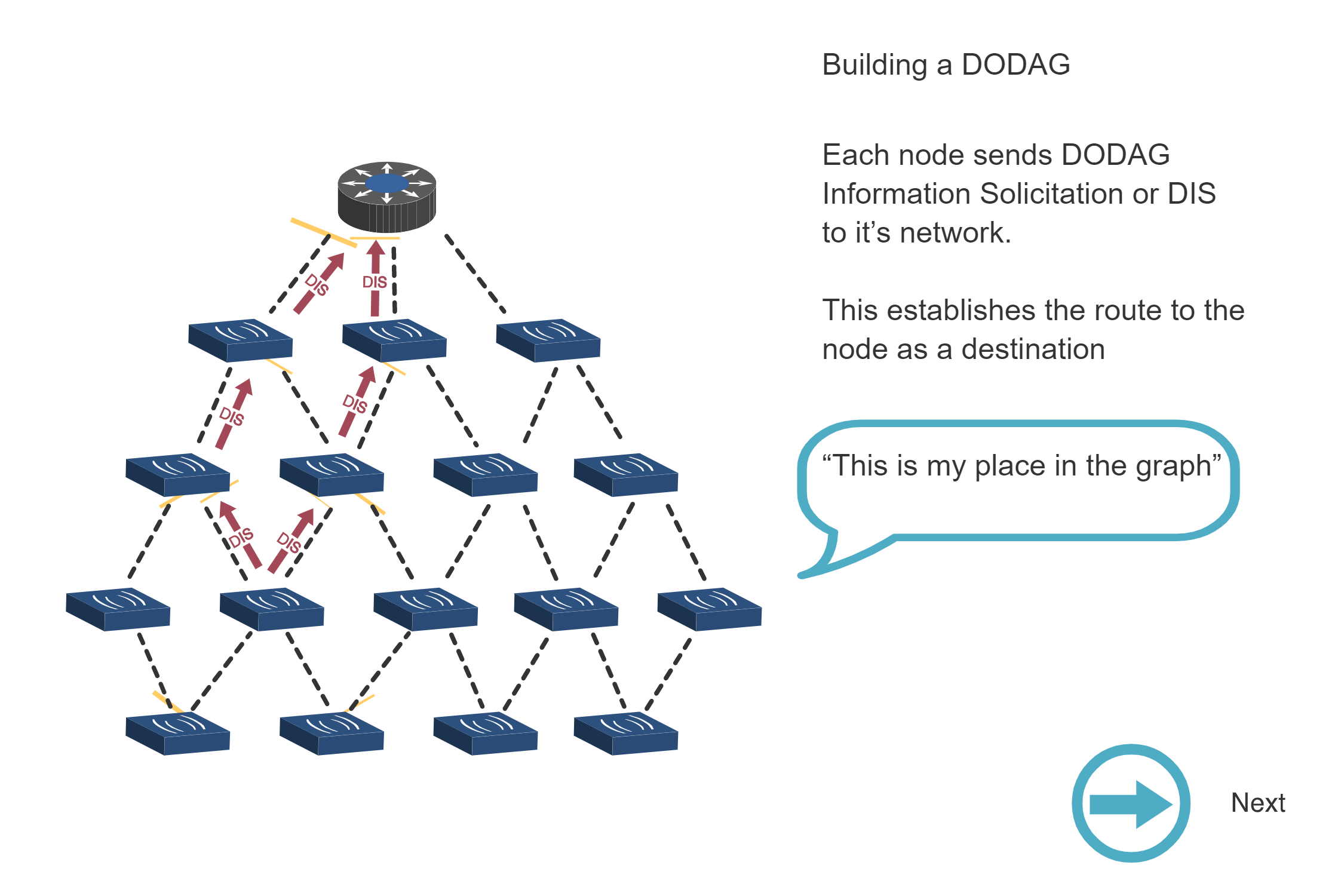
- Some nodes send DIS (DODAG Information Solicitation):
- Message content: “Hello? Is there a DODAG here? Send me DIO!”
- Purpose: Speed up discovery instead of waiting for periodic DIOs
- When sent: New node joining, or node woke from sleep and missed DIOs
- Response: Neighbors immediately reply with DIO messages
- Nodes receive DIOs from row 2 neighbors:
- Calculate their RANK:
RANK = parent_RANK + rank_increase(e.g., 256 + 200 = 456) - Select parent with best metrics (lowest RANK, good link quality)
- May hear DIOs from multiple potential parents
- Calculate their RANK:
- Nodes establish position in DODAG hierarchy:
- Store parent pointer, RANK value, DODAG_ID
- Determine which “floor” they’re on in the building analogy
Real-world timing: DIS accelerates joining from 10-30s (waiting for DIOs) to 2-5s (proactive request)
Trickle timer interaction: DIS resets trickle timer on recipients -> they send DIOs sooner -> faster convergence
715.3.2.5 Step 5: DAO Messages Flow Upward (t = 10-20 seconds)
All Nodes Send DAO to Build Downward Routes
Now that all nodes have joined and selected parents, they advertise their reachability:
- All nodes send DAO upward toward root:
- Leaf nodes send DAO to their parents
- Intermediate nodes aggregate DAOs from children and forward upward
- Storing mode: Each parent stores “Node X reachable via child Y”
- Non-Storing mode: Only root stores complete topology
- DAOs propagate upward hop-by-hop:
- Row 4 -> Row 3 -> Row 2 -> Root
- Each hop adds routing information
- Purpose: Build downward routes so root/parents can send packets to specific nodes
Real-world timing: DAO messages sent every 30-60 seconds (controlled by DAO timer)
Overhead: In 50-node network, ~50 DAO messages total (one per node) over 10-20 seconds
715.3.2.6 Step 6: Root Confirms Routes (t = 20-30 seconds)
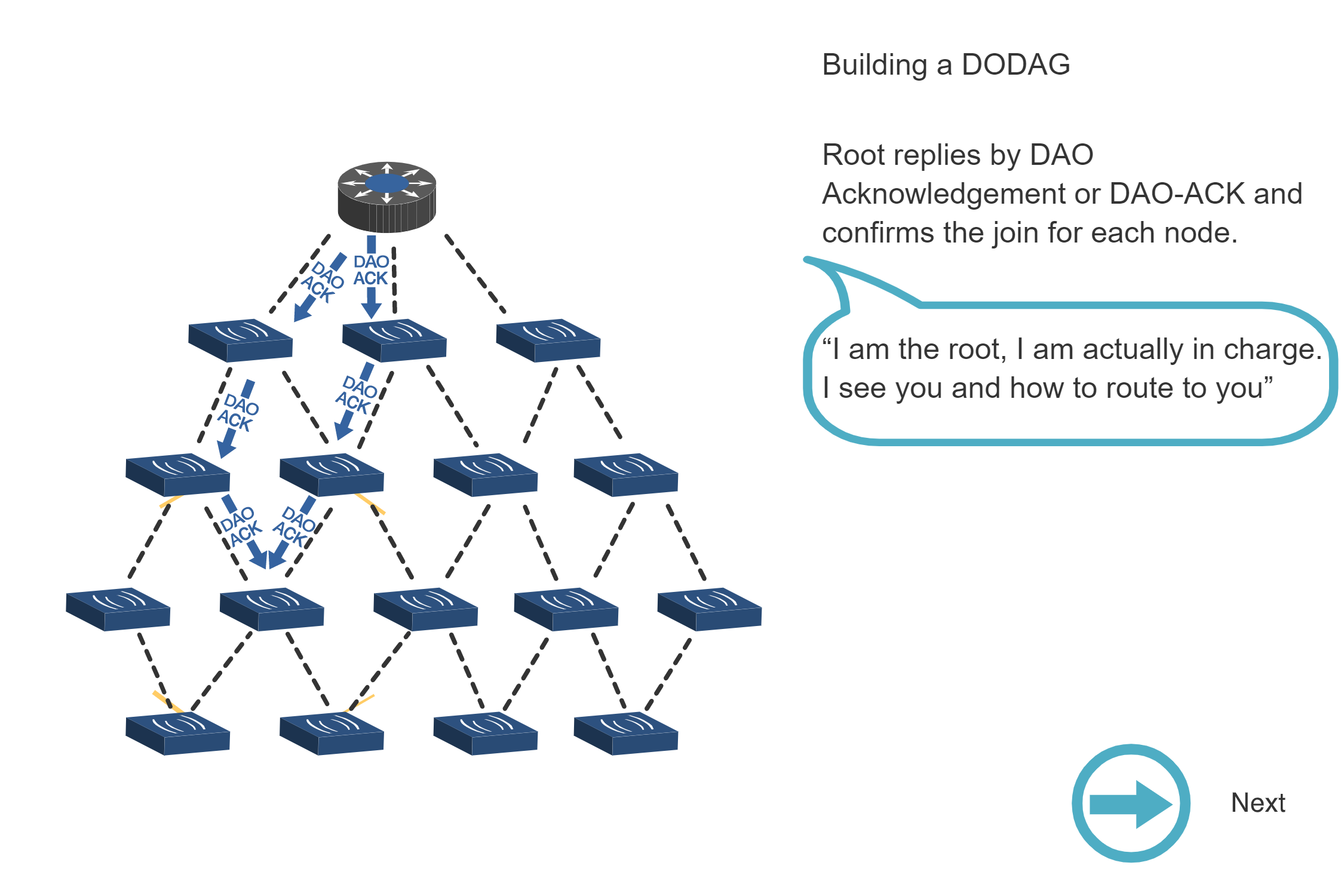
Root Sends DAO-ACK Confirmations
Root (or parents in Storing mode) send DAO-ACK to acknowledge DAO messages:
- Message content: “I received your DAO, I know how to reach you now”
- Direction: Parent -> Child (downward, following the DAO path in reverse)
- Purpose:
- Reliability: Confirm routing table updated successfully
- Error detection: If DAO-ACK doesn’t arrive, node retransmits DAO after timeout
- Root authority: “I am the root, I see you and know how to route to you”
- Optional: DAO-ACK can be disabled in low-reliability networks to reduce overhead
Real-world timing: DAO-ACK sent immediately after receiving DAO (1-2 seconds)
Storing vs Non-Storing: In Storing mode, each parent sends DAO-ACK. In Non-Storing mode, only root sends DAO-ACK (since only root stores routes).
715.3.2.7 Step 7: Steady State - DODAG Complete (t = 30+ seconds)
DODAG Formation Complete! Network is now operational with bidirectional routing:
- Upward routes (sensors -> root): Each node knows its parent (parent pointer)
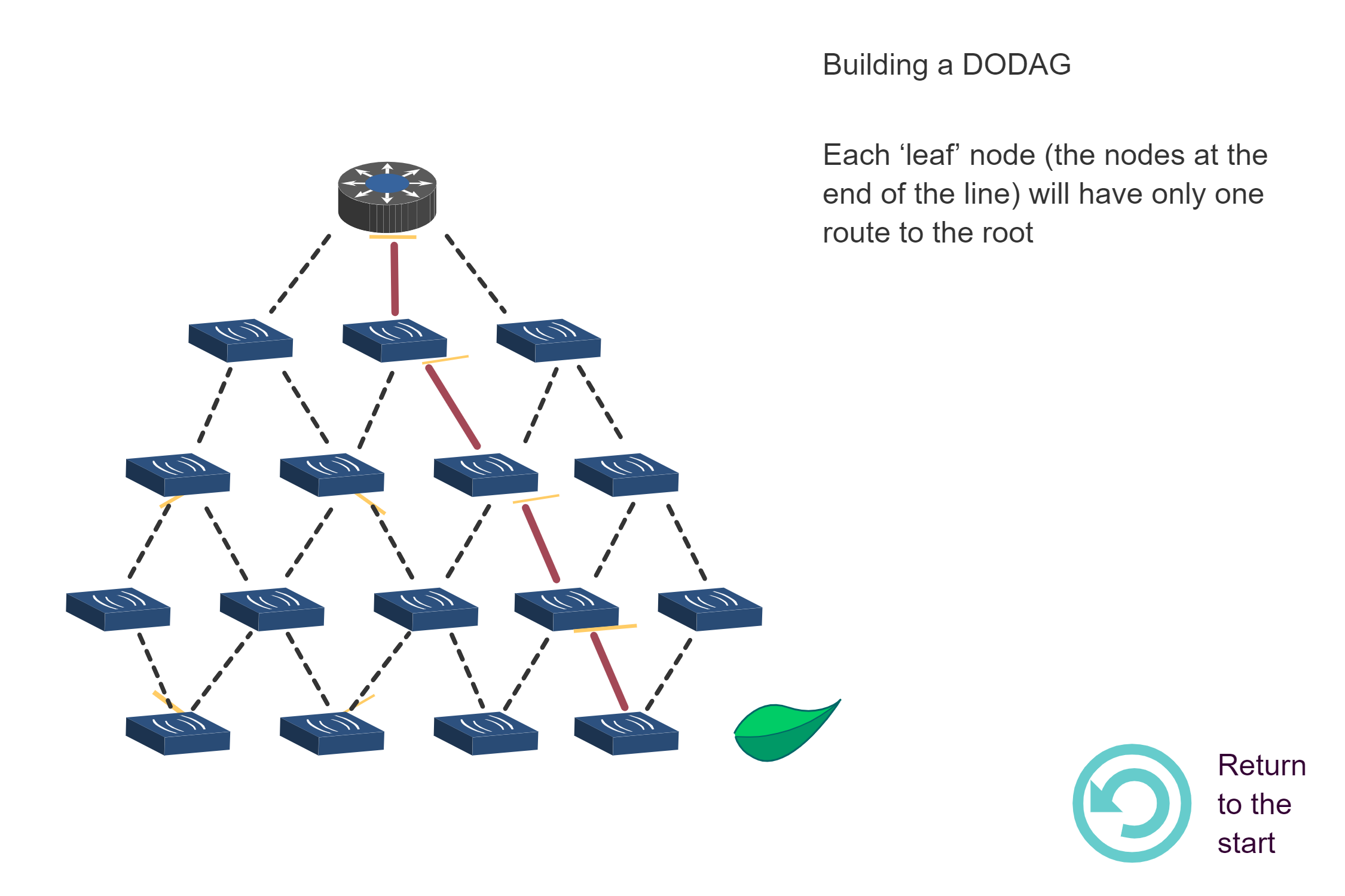
- Leaf nodes have one primary parent (solid line in diagram)
- Intermediate nodes may store backup parents (dotted lines = alternate paths)
- Default route: “Send to parent” (no routing table needed for upward)
- Memory: 4-8 bytes per node (just parent pointer)
- Downward routes (root -> sensors): Built via DAO messages
- Storing mode: Each node has routing table for descendants (10-100 KB total)
- Non-Storing mode: Only root has routing table, uses source routing (root needs 10-100 KB, nodes need 0 bytes)
- Network operational: Data can flow:
- Upward: Sensor readings -> cloud (many-to-one)
- Downward: Commands/firmware -> actuators (one-to-many)
- Point-to-point: Sensor <-> actuator via common ancestor
Key observation: Leaf nodes (bottom row) have one primary route to root, but network maintains alternate paths (dotted lines) for fault tolerance. If primary parent fails, node switches to backup parent instantly (no global reconfiguration needed).
Maintenance overhead: After convergence, trickle timer backs off to 10-60 minute DIO intervals, using <1% of bandwidth
715.4 DODAG Formation Timing Summary
Understanding the temporal progression helps you diagnose network formation issues and optimize convergence time:
| Step | Time | Action | Key Timing Factors |
|---|---|---|---|
| 1. Initial | t=0s | Unorganized network | Power-on, all nodes listening |
| 2. Root DIO | t=0-2s | Root broadcasts first DIO | Immediate on startup |
| 3. First-hop join | t=2-5s | Row 2 joins, sends DAO+DIO | DIO processing + RANK calc |
| 4. Ripple expansion | t=5-10s | Rows 3-4 join via DIS/DIO | DIS accelerates (vs waiting for periodic DIO) |
| 5. DAO upward | t=10-20s | All nodes send DAO to root | DAO timer (30-60s default, can be faster) |
| 6. DAO-ACK confirm | t=20-30s | Root confirms all routes | ACK sent immediately after DAO |
| 7. Steady state | t=30s+ | Network operational | Trickle backs off to 10-60 min DIOs |
Convergence time for 50-node network: Typically 30-120 seconds depending on: - Trickle timer settings: Aggressive (Imin=10ms) vs conservative (Imin=1s) - Network depth: 3-hop network converges faster than 7-hop - DIS usage: Proactive DIS reduces convergence from 120s to 30s - Radio conditions: Packet loss increases retransmissions and delays
Critical applications: Use aggressive timers (10s convergence), accept higher control overhead
Battery-optimized deployments: Tolerate slower formation (2-5 min), minimize DIO/DAO frequency
715.5 Complete DODAG Formation Overview
Summary of DODAG Formation:
This comprehensive view shows the complete temporal evolution of RPL DODAG construction:
- Initial chaos -> Unorganized nodes with potential connections
- Root broadcast -> DIO messages establish DODAG identity (RANK 0)
- Upward advertisement -> DAO messages build downward routing paths
- Position discovery -> DIS messages accelerate node integration
- Route confirmation -> DAO-ACK validates routing table entries
- Final hierarchy -> Operational tree with fault-tolerant alternate paths
Key pedagogical insight: Understanding the process (how DODAG forms over time) is more important than memorizing the final topology. When troubleshooting RPL networks, you’ll diagnose issues by observing DIO/DAO/DIS message flows during formation, not by looking at static routing tables.
Real-world timing: In a 50-node sensor network, complete DODAG formation typically takes 30-120 seconds depending on trickle timer settings, radio conditions, and network depth (max hops from root). Critical applications use aggressive timers (10s convergence), while battery-optimized deployments tolerate slower formation (2-5 min) for reduced control overhead.
715.6 Summary
This chapter covered the visual progression of DODAG construction:
- 5-Phase Algorithm: Root init -> First-hop join -> Multi-hop expand -> DAO propagation -> Steady state
- DAG vs DODAG: DODAG has exactly one root destination, ideal for IoT many-to-one traffic
- 7-Step Formation: Detailed temporal progression from t=0s to steady state at t=30+s
- Timing Factors: Trickle settings, network depth, DIS usage, and radio conditions affect convergence
- Fault Tolerance: Backup parents enable instant failover without global reconfiguration
715.7 What’s Next
Continue learning about DODAG construction details:
- RPL DODAG Message Flow: Detailed message exchange sequences
- RPL DODAG Worked Example: Complete 10-node network calculation
- RPL Trickle Algorithm: Energy-efficient maintenance mechanism
- RPL DODAG Construction Overview: Return to overview