%%{init: {'theme': 'base', 'themeVariables': { 'primaryColor': '#2C3E50', 'primaryTextColor': '#fff', 'primaryBorderColor': '#16A085', 'lineColor': '#16A085', 'secondaryColor': '#E67E22', 'tertiaryColor': '#7F8C8D'}}}%%
graph TB
    A["Node A"]
    B["Node B"]
    C["Node C"]
    D["Node D"]
    E["Node E"]

    A --> B
    A --> C
    B --> D
    C --> D
    D --> E

    style A fill:#2C3E50,stroke:#16A085,color:#fff
    style B fill:#16A085,stroke:#2C3E50,color:#fff
    style C fill:#16A085,stroke:#2C3E50,color:#fff
    style D fill:#E67E22,stroke:#2C3E50,color:#fff
    style E fill:#7F8C8D,stroke:#2C3E50,color:#fff
698 RPL Core Concepts and DODAG Construction
698.1 RPL Core Concepts
698.1.1 Directed Acyclic Graph (DAG)
DAG = Directed Acyclic Graph
{fig-alt=“Directed Acyclic Graph (DAG) example showing nodes A through E connected with directed arrows flowing downward, demonstrating no cycles - cannot return to same node following edges”}
Key Properties: - Directed: Edges have direction (arrows) - Acyclic: No cycles (cannot return to same node following edges) - Graph: Nodes connected by edges
Why DAG? - Loop-free routing: By definition, no cycles = no routing loops - Hierarchical structure: Natural parent-child relationships - Efficient aggregation: Data flows towards root(s)
698.1.2 DODAG (Destination Oriented DAG)
RPL uses DODAG: DAG with single root (destination)
%%{init: {'theme': 'base', 'themeVariables': { 'primaryColor': '#2C3E50', 'primaryTextColor': '#fff', 'primaryBorderColor': '#16A085', 'lineColor': '#16A085', 'secondaryColor': '#E67E22', 'tertiaryColor': '#7F8C8D'}}}%%
graph TB
    ROOT["ROOT<br/>(Single Destination)<br/>Rank: 0"]
    A["Node A<br/>Rank: 256"]
    B["Node B<br/>Rank: 256"]
    C["Node C<br/>Rank: 512"]
    D["Node D<br/>Rank: 512"]
    E["Node E<br/>Rank: 768"]
    F["Node F<br/>Rank: 768"]

    ROOT --> A
    ROOT --> B
    A --> C
    A --> D
    B --> D
    C --> E
    D --> F

    style ROOT fill:#2C3E50,stroke:#16A085,color:#fff,stroke-width:4px
    style A fill:#16A085,stroke:#2C3E50,color:#fff
    style B fill:#16A085,stroke:#2C3E50,color:#fff
    style C fill:#E67E22,stroke:#2C3E50,color:#fff
    style D fill:#E67E22,stroke:#2C3E50,color:#fff
    style E fill:#7F8C8D,stroke:#2C3E50,color:#fff
    style F fill:#7F8C8D,stroke:#2C3E50,color:#fff
{fig-alt=“Destination Oriented Directed Acyclic Graph (DODAG) with single ROOT node at top (Rank 0), intermediate nodes at Rank 256 and 512, leaf nodes at Rank 768, all paths flowing toward root”}
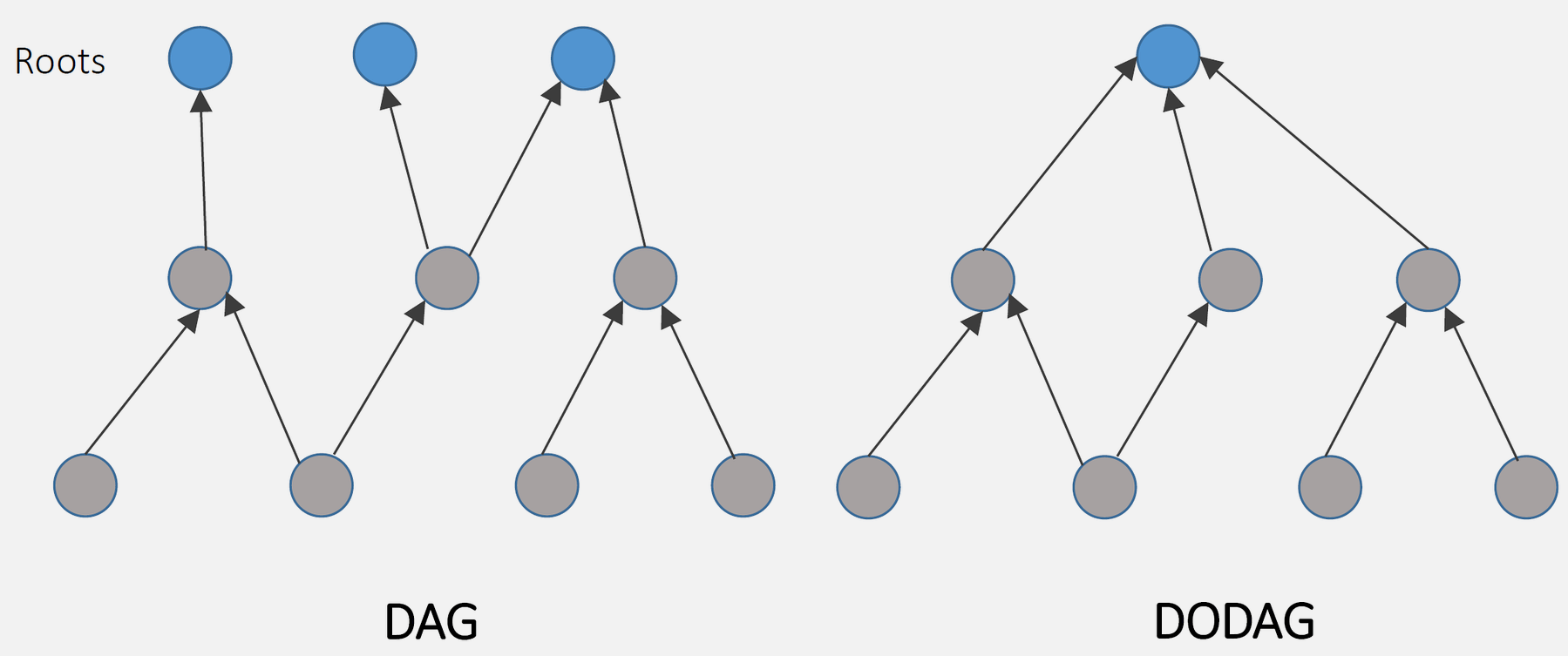
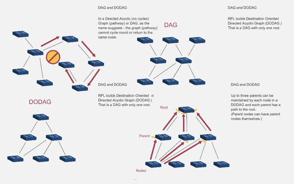
DODAG Properties: - Single root: One destination (typically border router/gateway) - Upward routes: All paths lead to root - RANK: Position in DODAG hierarchy (root = 0, increases going down)
698.1.3 RANK: Loop Prevention Mechanism
RANK is a scalar representing a node’s position relative to the root.
%%{init: {'theme': 'base', 'themeVariables': { 'primaryColor': '#2C3E50', 'primaryTextColor': '#fff', 'primaryBorderColor': '#16A085', 'lineColor': '#16A085', 'secondaryColor': '#E67E22', 'tertiaryColor': '#7F8C8D'}}}%%
graph TB
    ROOT["ROOT<br/>RANK = 0"]
    A["Node A<br/>RANK = 100"]
    B["Node B<br/>RANK = 250"]
    C["Node C<br/>RANK = 370"]

    ROOT -->|"Good link<br/>+100"| A
    A -->|"Poor link<br/>+150"| B
    B -->|"Good link<br/>+120"| C

    C -.->|"❌ Cannot choose<br/>(370 > 100 = loop!)"| A

    style ROOT fill:#2C3E50,stroke:#16A085,color:#fff,stroke-width:4px
    style A fill:#16A085,stroke:#2C3E50,color:#fff
    style B fill:#E67E22,stroke:#2C3E50,color:#fff
    style C fill:#7F8C8D,stroke:#2C3E50,color:#fff
{fig-alt=“RANK loop prevention mechanism showing ROOT at Rank 0, Node A at 100, B at 250, C at 370, with valid forward links and forbidden backward link from C to A that would create a loop”}
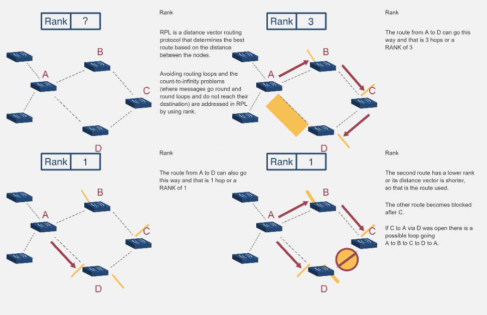
RANK Rules: 1. Root has RANK 0 (or minimum RANK) 2. RANK increases as you move away from root 3. Upward routing: Packets forwarded to nodes with lower RANK 4. Loop prevention: Node cannot choose parent with higher RANK
RANK Calculation:
RANK(node) = RANK(parent) + RankIncrease

RankIncrease calculated based on:
- Link cost (ETX, RSSI, etc.)
- Number of hops
- Energy consumed
- Objective functionExample:
ROOT: RANK = 0
Node A (parent: ROOT): RANK = 0 + 100 = 100
Node B (parent: Node A): RANK = 100 + 150 = 250
Node C (parent: Node B): RANK = 250 + 120 = 370
Loop Prevention: - Node C cannot choose Node A as parent (RANK 100 < 370 is OK) - Node A cannot choose Node C as parent (RANK 370 > 100 - would create loop)
ImportantRANK vs Hop Count
RANK ≠ Hop Count (although hop count can be a factor)
RANK is calculated using objective function which may consider: - Hop count - Expected Transmission Count (ETX) - Latency - Energy consumption - Link quality (RSSI, LQI)
Example: - Good link, 1 hop: RANK increase = 100 - Poor link, 1 hop: RANK increase = 300 - Good link, 2 hops: RANK increase = 200
Node may prefer 2 hops via good links (total RANK increase: 200) over 1 hop via poor link (RANK increase: 300).
698.2 DODAG Construction Process
RPL builds the DODAG through control messages:
%%{init: {'theme': 'base', 'themeVariables': { 'primaryColor': '#2C3E50', 'primaryTextColor': '#fff', 'primaryBorderColor': '#16A085', 'lineColor': '#16A085', 'secondaryColor': '#E67E22', 'tertiaryColor': '#7F8C8D'}}}%%
graph TB
    DIO["DIO<br/>DODAG Information Object<br/>Advertise DODAG"]
    DIS["DIS<br/>DODAG Information Solicitation<br/>Request DODAG info"]
    DAO["DAO<br/>Destination Advertisement Object<br/>Advertise reachability"]
    DAOACK["DAO-ACK<br/>Acknowledge DAO"]

    ROOT["ROOT sends DIO"]
    NODE["Node receives DIO"]
    JOIN["Node joins DODAG"]
    ADV["Node sends DAO"]

    ROOT --> NODE
    NODE --> JOIN
    JOIN --> ADV

    style DIO fill:#2C3E50,stroke:#16A085,color:#fff,stroke-width:3px
    style DIS fill:#16A085,stroke:#2C3E50,color:#fff
    style DAO fill:#E67E22,stroke:#2C3E50,color:#fff
    style DAOACK fill:#7F8C8D,stroke:#2C3E50,color:#fff
    style ROOT fill:#2C3E50,stroke:#16A085,color:#fff
    style NODE fill:#16A085,stroke:#2C3E50,color:#fff
    style JOIN fill:#E67E22,stroke:#2C3E50,color:#fff
    style ADV fill:#7F8C8D,stroke:#2C3E50,color:#fff
{fig-alt=“RPL control messages overview showing DIO (advertise DODAG), DIS (request info), DAO (advertise reachability), DAO-ACK (acknowledgment), and DODAG construction flow from ROOT sending DIO through node joining to DAO advertisement”}
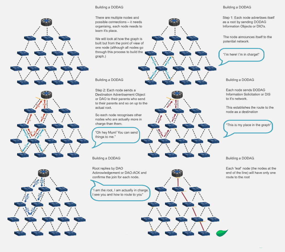
698.2.1 Step-by-Step DODAG Construction
%%{init: {'theme': 'base', 'themeVariables': { 'primaryColor': '#2C3E50', 'primaryTextColor': '#fff', 'primaryBorderColor': '#16A085', 'lineColor': '#16A085', 'secondaryColor': '#E67E22', 'tertiaryColor': '#7F8C8D'}}}%%
sequenceDiagram
    participant ROOT as ROOT (Rank 0)
    participant N1 as Node 1
    participant N2 as Node 2
    participant N3 as Node 3

    Note over ROOT: Step 1: ROOT initiates DODAG
    ROOT->>ROOT: Create DODAG ID<br/>Set RANK = 0
    ROOT->>N1: DIO (DODAG_ID, RANK=0)
    ROOT->>N2: DIO (DODAG_ID, RANK=0)

    Note over N1,N2: Step 2: Nodes receive DIO and join
    N1->>N1: Calculate RANK = 100<br/>Select ROOT as parent
    N2->>N2: Calculate RANK = 100<br/>Select ROOT as parent

    Note over N1,N2: Step 3: Nodes propagate DIO
    N1->>N3: DIO (DODAG_ID, RANK=100)
    N2->>N3: DIO (DODAG_ID, RANK=100)

    Note over N3: Step 4: Build upward routes
    N3->>N3: Calculate RANK = 200<br/>Select N1 as parent<br/>Parent pointer established

    Note over N3: Step 5: Build downward routes
    N3->>N1: DAO (I am reachable)
    N1->>ROOT: DAO (N3 reachable via me)
    ROOT->>N1: DAO-ACK
{fig-alt=“DODAG construction sequence diagram showing 5 steps: ROOT initiates with DIO, nodes receive and join calculating RANK, nodes propagate DIO, upward routes established via parent pointers, downward routes built via DAO messages”}
698.2.2 Detailed Construction Steps
NoteStep 1: Root Initiates DODAG
Root node (border router/gateway): 1. Creates DODAG: Assigns unique DODAG ID 2. Sets RANK = 0: Root has minimum RANK 3. Broadcasts DIO: Sends DODAG Information Object (multicast)
DIO Contents: - DODAG ID (IPv6 address) - RANK (0 for root) - Objective function (routing metric) - DODAG configuration (timers, etc.)
698.3 Step 2: Nodes Receive DIO and Join
Node receives DIO: 1. Decision: Join this DODAG or wait for others? - Compare DODAG rank, objective function - May receive DIOs from multiple DODAGs 2. Calculate RANK: RANK = parent_RANK + increase 3. Select parent: Choose sender of DIO (if acceptable) 4. Update state: Store DODAG ID, parent, RANK
Multiple DIO Sources: - Node may hear DIOs from multiple neighbors - Chooses best parent (lowest RANK, best link quality) - May maintain backup parents (loop-free)
698.4 Step 3: Nodes Propagate DIO
After joining DODAG: 1. Node becomes part of DODAG 2. Sends own DIO: Advertises DODAG to neighbors 3. DIO contents: Own RANK, DODAG ID, etc. 4. Trickle timer: Controls DIO frequency (adaptive)
Trickle Algorithm: - Stable network: Send DIOs infrequently (minutes) - Network changes: Send DIOs frequently (seconds) - Reduces overhead while maintaining responsiveness
NoteStep 4: Build Upward Routes
Upward routes (towards root) established automatically: - Each node knows its parent (from DIO selection) - Default route: Send to parent (towards root) - No routing table needed for upward routes (just parent pointer)
Example:
Node 3 → Node 1 → Root
(N3 knows parent is N1, N1 knows parent is Root)
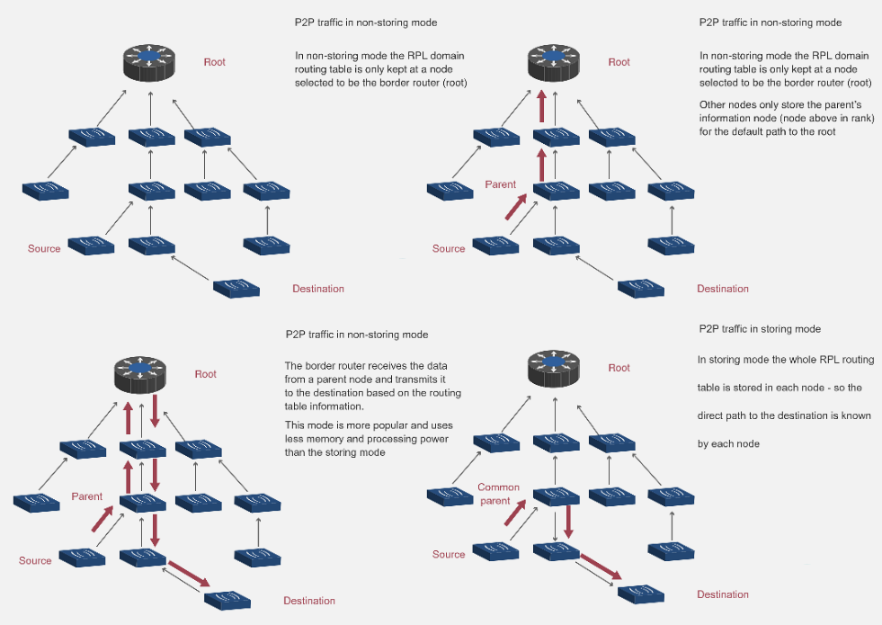
NoteStep 5: Build Downward Routes (Storing Mode)
Downward routes (from root to nodes) require DAO messages:
- Node sends DAO to parent:
- “I am reachable via you”
- Includes node’s address and prefixes
- Parent updates routing table:
- “Node X is reachable via this child”
- Parent propagates DAO towards root:
- Aggregates reachability information
- Root knows all nodes:
- Complete routing table for downward routes
DAO-ACK (optional): - Parent confirms DAO receipt - Reliability for critical networks