%%{init: {'theme': 'base', 'themeVariables': { 'primaryColor': '#2C3E50', 'primaryTextColor': '#fff', 'primaryBorderColor': '#16A085', 'lineColor': '#E67E22', 'secondaryColor': '#16A085', 'tertiaryColor': '#E8F6F3', 'clusterBkg': '#E8F6F3', 'clusterBorder': '#16A085', 'fontSize': '13px'}}}%%
graph LR
    File["Large File<br/>1 MB"]
    D1["Datagram 1<br/>1500 bytes"]
    D2["Datagram 2<br/>1500 bytes"]
    D3["Datagram 3<br/>1500 bytes"]
    D4["..."]
    D5["Datagram N<br/>1500 bytes"]

    File -->|Break into<br/>packets| D1
    File --> D2
    File --> D3
    File --> D4
    File --> D5

    style File fill:#2C3E50,stroke:#16A085,color:#fff
    style D1 fill:#16A085,stroke:#2C3E50,color:#fff
    style D2 fill:#E67E22,stroke:#2C3E50,color:#fff
    style D3 fill:#16A085,stroke:#2C3E50,color:#fff
    style D4 fill:#7F8C8D,stroke:#2C3E50,color:#fff
    style D5 fill:#16A085,stroke:#2C3E50,color:#fff
644 Datagrams and Packet Structure
644.1 Learning Objectives
By the end of this section, you will be able to:
- Define Datagram Structure: Explain the components of a network datagram (header and payload)
- Describe Packet Headers: Identify key header fields including addresses, sequence numbers, and checksums
- Understand Encapsulation: Explain how each protocol layer adds its own header to data
- Evaluate Fragmentation: Understand why large data must be broken into smaller packets
644.2 Prerequisites
Before diving into this chapter, you should be familiar with:
- Data Representation in Networks: Understanding bits, bytes, and data sizes
- Networking Basics: Core networking concepts and terminology
ImportantWhy Datagrams Matter for IoT
Every IoT message is a datagram. Whether your temperature sensor sends a 10-byte reading or your security camera streams video, all data travels as packets with headers and payloads. Understanding this structure helps you debug network issues, optimize bandwidth usage, and choose appropriate protocols.
TipFor Beginners: Understanding Packets
Imagine sending a book page-by-page through the mail instead of as one heavy package. Each page (packet) gets its own envelope with: - Sender’s address (who sent it) - Recipient’s address (who receives it) - Page number (sequence for reassembly) - The actual content (one page of the book)
Networks work the same way - large files are broken into small packets, each labeled with addressing and ordering information. At the destination, packets are reassembled into the original file, even if they arrived out of order or took different routes.
644.3 What is a Datagram?
The key to data communications: The data stream is broken into small pieces.
{fig-alt=“Diagram showing large 1 MB file broken into multiple 1500-byte datagrams for network transmission”}
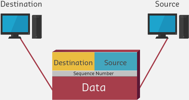
Each datagram consists of:
- Header (label with control information):
- Source address: Where it came from
- Destination address: Where it’s going
- Sequence number: Order in original data
- Protocol information: How to process it
- Error checking: Verify data integrity
- Payload (actual data):
- Sensor readings
- Commands
- File fragments
- Video frames
644.4 Datagram Structure
%%{init: {'theme': 'base', 'themeVariables': { 'primaryColor': '#2C3E50', 'primaryTextColor': '#fff', 'primaryBorderColor': '#16A085', 'lineColor': '#E67E22', 'secondaryColor': '#16A085', 'tertiaryColor': '#E8F6F3', 'clusterBkg': '#E8F6F3', 'clusterBorder': '#16A085', 'fontSize': '12px'}}}%%
graph TB
    subgraph Datagram["Datagram / Packet"]
        subgraph Header["Header (20-60 bytes)"]
            Src["Source Address<br/>192.168.1.100"]
            Dst["Destination Address<br/>54.235.123.45"]
            Seq["Sequence Number<br/>#1 of 100"]
            Proto["Protocol<br/>TCP/UDP"]
            CRC["Error Check<br/>CRC/Checksum"]
        end
        subgraph Payload["Payload (46-1460 bytes)"]
            Data["Actual Data<br/>Temperature: 23.5C<br/>Humidity: 65%<br/>..."]
        end
    end

    style Src fill:#2C3E50,stroke:#16A085,color:#fff
    style Dst fill:#16A085,stroke:#2C3E50,color:#fff
    style Seq fill:#E67E22,stroke:#2C3E50,color:#fff
    style Proto fill:#2C3E50,stroke:#16A085,color:#fff
    style CRC fill:#16A085,stroke:#2C3E50,color:#fff
    style Data fill:#E67E22,stroke:#2C3E50,color:#fff
{fig-alt=“Detailed datagram packet structure showing header components (source/destination addresses, sequence number, protocol type, error checking) and payload section with actual sensor data”}
Why use datagrams? - Flexibility: Multiple paths can be used simultaneously - Efficiency: Share network infrastructure across many users - Resilience: Reroute around failures - Error recovery: Retransmit only lost pieces, not entire file
644.5 Protocol Encapsulation
As data passes through protocol layers, each layer adds its own header. This process is called encapsulation.
TipAlternative View: Datagram Journey Through Protocol Layers
This variant shows how a datagram is built as it passes through protocol layers (encapsulation):
%%{init: {'theme': 'base', 'themeVariables': { 'primaryColor': '#2C3E50', 'primaryTextColor': '#fff', 'primaryBorderColor': '#16A085', 'lineColor': '#E67E22', 'secondaryColor': '#16A085'}}}%%
graph TB
    subgraph APP["Application Layer"]
        D1["Temperature: 23.5C"]
    end

    subgraph TRANS["Transport Layer (UDP)"]
        D2["Port Header + Temperature: 23.5C"]
    end

    subgraph NET["Network Layer (IP)"]
        D3["IP Header + Port Header + Data"]
    end

    subgraph LINK["Data Link (Ethernet)"]
        D4["MAC Header + IP + Port + Data + FCS"]
    end

    APP -->|"Add port numbers"| TRANS
    TRANS -->|"Add IP addresses"| NET
    NET -->|"Add MAC + checksum"| LINK

    SIZE1["5 bytes"]
    SIZE2["13 bytes"]
    SIZE3["33 bytes"]
    SIZE4["51+ bytes"]

    D1 --- SIZE1
    D2 --- SIZE2
    D3 --- SIZE3
    D4 --- SIZE4

    style D1 fill:#E67E22,stroke:#2C3E50,color:#fff
    style D2 fill:#16A085,stroke:#2C3E50,color:#fff
    style D3 fill:#2C3E50,stroke:#16A085,color:#fff
    style D4 fill:#2C3E50,stroke:#16A085,color:#fff
    style SIZE1 fill:#7F8C8D,stroke:#2C3E50,color:#fff
    style SIZE2 fill:#7F8C8D,stroke:#2C3E50,color:#fff
    style SIZE3 fill:#7F8C8D,stroke:#2C3E50,color:#fff
    style SIZE4 fill:#7F8C8D,stroke:#2C3E50,color:#fff
Each layer adds its own header (encapsulation), growing the datagram from a simple 5-byte sensor value to a 51+ byte frame on the wire.
644.5.1 Encapsulation in Practice
When your IoT sensor sends “Temperature: 23.5C” (about 5 bytes of data):
| Layer | Header Added | Running Total |
|---|---|---|
| Application | None (raw data) | 5 bytes |
| Transport (UDP) | 8-byte UDP header | 13 bytes |
| Network (IP) | 20-byte IP header | 33 bytes |
| Data Link (Ethernet) | 18-byte Ethernet + FCS | 51+ bytes |
Your 5-byte sensor reading becomes a 51-byte frame - 90% overhead!
This is why IoT protocols like CoAP use UDP (8-byte header) instead of TCP (20-byte header), and why binary encoding (2-4 bytes for temperature) is preferred over JSON (~20 bytes for {"temp":23.5}).
644.6 Circuit Switching vs Packet Switching
Understanding datagrams requires contrasting them with the older approach - circuit switching.
TipAlternative View: Circuit Switching vs Packet Switching
This variant compares the old telephone network model (circuit switching) with modern Internet model (packet switching):
%%{init: {'theme': 'base', 'themeVariables': { 'primaryColor': '#2C3E50', 'primaryTextColor': '#fff', 'primaryBorderColor': '#16A085', 'lineColor': '#E67E22', 'secondaryColor': '#16A085'}}}%%
graph TB
    subgraph CIRCUIT["Circuit Switching (Old Phones)"]
        C1["Caller A"] -->|"Dedicated path<br/>Reserved for duration"| C2["Receiver B"]
        CN["Resources: 100%<br/>even during silence"]
    end

    subgraph PACKET["Packet Switching (Internet/IoT)"]
        P1["Device A"] -->|"Packet 1"| R1["Router"]
        P1 -->|"Packet 2"| R2["Router"]
        R1 -->|"Mixed with<br/>other traffic"| P2["Device B"]
        R2 --> P2
        PN["Resources: Only<br/>when transmitting"]
    end

    EFFICIENCY["Packet Switching: 10-100x more<br/>efficient for bursty IoT traffic"]

    CIRCUIT --> EFFICIENCY
    PACKET --> EFFICIENCY

    style C1 fill:#7F8C8D,stroke:#2C3E50,color:#fff
    style C2 fill:#7F8C8D,stroke:#2C3E50,color:#fff
    style CN fill:#7F8C8D,stroke:#2C3E50,color:#fff
    style P1 fill:#16A085,stroke:#2C3E50,color:#fff
    style R1 fill:#E67E22,stroke:#2C3E50,color:#fff
    style R2 fill:#E67E22,stroke:#2C3E50,color:#fff
    style P2 fill:#16A085,stroke:#2C3E50,color:#fff
    style PN fill:#16A085,stroke:#2C3E50,color:#fff
    style EFFICIENCY fill:#2C3E50,stroke:#16A085,color:#fff
IoT devices send data in bursts (a sensor reading every minute). Packet switching only uses network resources during actual transmission, making it ideal for IoT.
| Aspect | Circuit Switching | Packet Switching |
|---|---|---|
| Resource Usage | Reserved entire duration | Only during transmission |
| Efficiency | Low for bursty traffic | High for bursty traffic |
| Failure Handling | Call drops if path fails | Packets reroute automatically |
| Example | Traditional phone calls | Internet, IoT networks |
For IoT: A temperature sensor that sends 100 bytes every 60 seconds would waste 99.99% of a dedicated circuit. Packet switching lets thousands of such devices share the same network efficiently.
644.7 Maximum Transmission Unit (MTU)
The Maximum Transmission Unit (MTU) defines the largest packet a network can handle:
| Network Type | Typical MTU | IoT Relevance |
|---|---|---|
| Ethernet | 1500 bytes | Standard for gateways |
| Wi-Fi | 2304 bytes | Smart home devices |
| IPv6 minimum | 1280 bytes | Guaranteed delivery |
| LoRaWAN | 51-242 bytes | Long-range sensors |
| 6LoWPAN | 127 bytes | Mesh sensors |
When data exceeds MTU, it must be fragmented into smaller packets. Fragmentation adds overhead and complexity, so IoT protocols are designed around constrained MTUs.
644.8 Knowledge Check
TipUnderstanding Check: Protocol Overhead and Efficiency
Scenario: Your IoT temperature sensor needs to transmit 1000 bytes of sensor data over a 100 Mbps Ethernet network. The networking stack adds 78 bytes of protocol overhead to each packet: preamble (8 bytes), MAC header (14 bytes), IP header (20 bytes), TCP header (20 bytes), CRC checksum (4 bytes), and inter-frame gap (12 bytes).
Transmission details: Total packet = 1000 bytes payload + 78 bytes overhead = 1078 bytes = 8624 bits
Think about: 1. What percentage of the bandwidth actually delivers useful sensor data versus protocol overhead? 2. If you were designing a low-power IoT sensor that transmits small 50-byte readings every 5 minutes, how would protocol overhead affect your design decisions?
Key Insight: Protocol efficiency = (Payload / Total packet size) x 100 = (1000 / 1078) x 100 = 92.8%. Transmission time = Total bits / Bandwidth = 8624 bits / (100 x 10^6 bps) = 86.24 microseconds. This means your goodput (usable data rate) is 92.8 Mbps of the 100 Mbps bandwidth - 7.2% is consumed by protocol overhead. The key insight: overhead is fixed per packet, regardless of payload size. A 1000-byte payload achieves 92.8% efficiency, but a 100-byte payload would achieve only 56% efficiency (100 / 178), and a 50-byte payload drops to 39% efficiency (50 / 128). This demonstrates why packet aggregation - combining multiple small sensor readings into larger packets - dramatically improves network efficiency for IoT deployments.
Question: An IoT sensor needs to send 1000 bytes of data over a 100 Mbps network. The protocol overhead is 78 bytes (headers, CRC, inter-frame gap). What is the protocol efficiency and transmission time?
Explanation: Protocol efficiency = (Payload / Total packet size) x 100 = (1000 / 1078) x 100 = 92.8%. Transmission time = (Total bits / Bandwidth). Total packet = 1078 bytes = 8624 bits. Time = 8624 bits / (100 x 10^6 bps) = 86.24 microseconds. Goodput (usable data rate) = 1000 bytes / 86.24 microseconds = 92.8 Mbps of the 100 Mbps bandwidth. The 78-byte overhead (preamble 8, MAC header 14, IP header 20, TCP header 20, CRC 4, inter-frame gap 12) represents 7.2% reduction in efficiency. This demonstrates why larger payloads improve efficiency - overhead is fixed per packet, so 1000-byte payload is more efficient than 100-byte payload.
644.9 Summary
- Datagrams are self-contained packets with headers (addressing, sequencing, error checking) and payloads (actual data)
- Protocol encapsulation adds headers at each layer, growing a 5-byte sensor reading to 51+ bytes on the wire
- Packet switching is dramatically more efficient than circuit switching for bursty IoT traffic
- MTU limits vary by network (1500 bytes for Ethernet, 51-242 bytes for LoRaWAN) and determine fragmentation needs
- Protocol efficiency depends on payload size - small packets have high overhead percentages, favoring aggregation
644.10 What’s Next
Now that you understand how data is packaged into datagrams, the next section explores how these packets are switched and routed through networks. You’ll learn about multiplexing, network resilience, and how routers make forwarding decisions.
Continue to: Packet Switching and Network Performance