Calculate free space path loss (FSPL) for various frequencies and distances
Apply the FSPL formula using both MHz/km and GHz/m conventions
Understand the log-distance path loss model for different environments
Interpret path loss exponents to characterize propagation environments
Estimate received signal strength from transmit power and path loss
634.2 Introduction
Understanding wireless signal propagation is critical for IoT deployments. Whether placing Wi-Fi access points, estimating LoRa range, or debugging BLE beacon issues, engineers must understand how radio waves behave in real environments.
Time: ~15 min | Difficulty: Intermediate | P07.C15.U05a
634.3 Why Propagation Matters for IoT
Real-World Problem: A smart building deploys 200 Zigbee temperature sensors with gateway placement based on theoretical 100m range specifications. After installation, 40% of sensors fail to connect. Post-mortem analysis reveals walls attenuate signals by 8-15 dB, reducing effective range to 30-50m.
Link margin: -48.03 - (-90) = 41.97 dB (excellent!)
Interpretation: At 50m in free space, Wi-Fi has 42 dB of margin. This extra margin accounts for fading, interference, and obstacles in real deployments.
Show code
{const container =document.getElementById('kc-net-5');if (container &&typeof InlineKnowledgeCheck !=='undefined') { container.innerHTML=''; container.appendChild(InlineKnowledgeCheck.create({question:"A LoRa sensor transmitting at 915 MHz is deployed 100m from a gateway. A Wi-Fi sensor transmitting at 2.4 GHz is deployed at the same 100m distance. Assuming free space path loss only, which signal experiences MORE attenuation and by approximately how much?",options: [ {text:"LoRa experiences ~8 dB more loss due to lower frequency",correct:false,feedback:"Lower frequency actually experiences LESS path loss, not more. The FSPL formula shows loss increases with frequency: FSPL = 20log(d) + 20log(f) + constant. Higher frequency = higher loss."}, {text:"Wi-Fi experiences ~8 dB more loss due to higher frequency",correct:true,feedback:"Correct! FSPL at 2.4 GHz vs 915 MHz: Difference = 20log(2400/915) = 20log(2.62) = 8.4 dB additional loss for Wi-Fi. This is why sub-GHz protocols like LoRa achieve longer range - they lose less signal to free space path loss."}, {text:"Both experience the same loss - distance is the only factor",correct:false,feedback:"The FSPL formula includes both distance AND frequency: FSPL = 20log(d) + 20log(f) + constant. At the same distance, higher frequency signals experience more path loss."}, {text:"Wi-Fi experiences ~20 dB more loss due to higher bandwidth",correct:false,feedback:"Bandwidth affects data rate and noise floor, not free space path loss. The ~8 dB difference comes from the 20log(f) term in the FSPL formula, not bandwidth considerations."} ],difficulty:"medium",topic:"Path Loss" })); }}
634.6 Worked Example: LoRa Long-Range Link Budget
Scenario: LoRaWAN sensor in rural farm environment at 915 MHz. What is maximum range?
Given: - Frequency: f = 915 MHz - Transmit power: 14 dBm (25 mW - regulatory limit US 915 MHz) - Receiver sensitivity: -137 dBm (LoRa SF12) - Required link margin: 10 dB (for fading)
Where: - L(d) = Path loss at distance d (dB) - L_0 = Path loss at reference distance d_0 (typically 1m) - n = Path loss exponent (environment-dependent) - d_0 = Reference distance (typically 1m) - X_sigma = Gaussian random variable for shadowing (dB)
Path Loss Exponents by Environment:
Environment
Path Loss Exponent (n)
Interpretation
Free space
n = 2.0
Ideal conditions
Urban cellular
n = 2.7 to 3.5
Buildings, reflections
Indoor office
n = 2.5 to 3.0
Cubicles, furniture
Indoor factory
n = 2.0 to 3.0
Open floor vs machinery
Indoor residential
n = 3.0 to 4.0
Walls, floors
Obstructed urban
n = 4.0 to 6.0
Dense buildings, no LOS
Key Insight: Higher path loss exponent = signal degrades faster with distance.
Figure 634.2: Signal strength degradation comparing free space, indoor office, and dense urban environments
{fig-alt=“Line chart comparing path loss versus distance for three environments: free space with n=2.0 showing slowest signal degradation, indoor office with n=3.0 showing moderate degradation, and dense urban with n=5.0 showing rapid signal attenuation, illustrating how environment affects wireless range”}
634.8 Summary
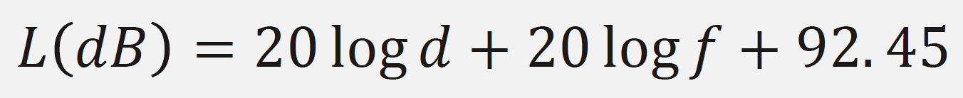
Free Space Path Loss (FSPL) provides the baseline for wireless range calculations using the formula: FSPL = 20log(d) + 20log(f) + constant
Higher frequencies experience more path loss - a 2.4 GHz signal loses ~8 dB more than a 915 MHz signal at the same distance
Path loss exponent (n) characterizes the environment: n=2 for free space, n=3-4 for indoor, n=4-6 for obstructed urban
Theoretical range far exceeds practical range - real deployments must account for environmental losses
Link budget analysis determines if a wireless connection will work by comparing received power to sensitivity
634.9 What’s Next
Continue to the Material Attenuation and RSSI chapter to learn how building materials affect signal strength and how RSSI is used for localization.