%% fig-cap: "Global Navigation Satellite Systems (GNSS) Overview"
%% fig-alt: "Diagram showing GNSS systems worldwide: GPS (USA), GLONASS (Russia), Galileo (EU), BeiDou (China)"

%%{init: {'theme': 'base', 'themeVariables': { 'primaryColor': '#2C3E50', 'primaryTextColor': '#fff', 'primaryBorderColor': '#16A085', 'lineColor': '#16A085', 'secondaryColor': '#E67E22', 'tertiaryColor': '#ecf0f1', 'noteTextColor': '#2C3E50', 'noteBkgColor': '#fff3cd', 'textColor': '#2C3E50', 'fontSize': '16px'}}}%%

graph TD
    GNSS[Global Navigation<br/>Satellite Systems]

    GNSS --> GPS[GPS - USA<br/>31 satellites<br/>5-10m accuracy]
    GNSS --> GLONASS[GLONASS - Russia<br/>24 satellites<br/>5-10m accuracy]
    GNSS --> Galileo[Galileo - EU<br/>30 satellites<br/>1-2m accuracy]
    GNSS --> BeiDou[BeiDou - China<br/>35 satellites<br/>5-10m accuracy]

    GPS --> Civilian[Civilian L1<br/>1575 MHz<br/>Public access]
    GPS --> Military[Military L2<br/>1227 MHz<br/>Encrypted]

    subgraph Characteristics["GNSS Characteristics"]
        Orbit[Medium Earth Orbit<br/>~20,000 km altitude]
        Coverage[Global Coverage<br/>4-12 satellites visible]
        Signal[Weak Signals<br/>10^-16 watts received]
    end

    style GNSS fill:#2C3E50,stroke:#16A085,stroke-width:4px,color:#fff
    style GPS fill:#16A085,stroke:#2C3E50,stroke-width:3px,color:#fff
    style GLONASS fill:#E67E22,stroke:#16A085,stroke-width:2px,color:#fff
    style Galileo fill:#16A085,stroke:#2C3E50,stroke-width:2px,color:#fff
    style BeiDou fill:#E67E22,stroke:#16A085,stroke-width:2px,color:#fff
1505 GPS and Outdoor Positioning
1505.1 Learning Objectives
By the end of this chapter, you will be able to:
- Explain GPS/GNSS Architecture: Understand the space, control, and user segments of satellite navigation systems
- Calculate Positioning from Satellites: Apply Time of Flight and TDoA principles to determine position
- Identify Multipath Effects: Recognize how signal reflections degrade positioning accuracy
- Understand Clock Synchronization: Explain why atomic clocks are essential and how pseudoranges work
1505.2 Prerequisites
- Location Awareness Fundamentals: Understanding of positioning technology landscape
1505.4 Time of Flight (ToF)
Time of Flight: Measure the time taken for a signal to propagate from transmitter to receiver.
%% fig-cap: "Time of Flight (ToF) Positioning Concept"
%% fig-alt: "Diagram showing Time of Flight positioning with signal transmission and distance calculation"

%%{init: {'theme': 'base', 'themeVariables': { 'primaryColor': '#2C3E50', 'primaryTextColor': '#fff', 'primaryBorderColor': '#16A085', 'lineColor': '#16A085', 'secondaryColor': '#E67E22', 'tertiaryColor': '#ecf0f1', 'noteTextColor': '#2C3E50', 'noteBkgColor': '#fff3cd', 'textColor': '#2C3E50', 'fontSize': '16px'}}}%%

graph LR
    Tx[Transmitter<br/>Satellite<br/>Time: T1]

    Tx -->|Signal travels at<br/>c = 299,792,458 m/s| Signal[RF Signal<br/>Time of Flight<br/>Δt = T2 - T1]

    Signal --> Rx[Receiver<br/>GPS Device<br/>Time: T2]

    Rx --> Calc[Distance Calculation<br/>d = c × Δt<br/>d = c × T2 - T1]

    Calc --> Result[Distance Result<br/>e.g., 20,000 km]

    subgraph Problem["Critical Challenge"]
        Sync[Clock Synchronization<br/>Required!<br/>1 μs error = 300m<br/>1 ns error = 0.3m]
    end

    style Tx fill:#2C3E50,stroke:#16A085,stroke-width:3px,color:#fff
    style Signal fill:#E67E22,stroke:#16A085,stroke-width:2px,color:#fff
    style Rx fill:#16A085,stroke:#2C3E50,stroke-width:3px,color:#fff
    style Calc fill:#2C3E50,stroke:#16A085,stroke-width:2px,color:#fff
    style Result fill:#16A085,stroke:#2C3E50,stroke-width:3px,color:#fff
    style Sync fill:#E67E22,stroke:#16A085,stroke-width:3px,color:#fff
Distance Calculation:
Distance = Speed of Light × Time of Flight
d = c × Δt

where:
- c = 299,792,458 m/s (speed of light in vacuum)
- Δt = reception time - transmission time
Critical Challenge: Both transmitter and receiver must have synchronized clocks to know the true transmission time.
Synchronization Sensitivity:
1 microsecond clock error = 300 meters position error!
1 nanosecond clock error = 0.3 meters position error
1505.5 The Multipath Problem
Multipath: Signals reflect off objects, creating multiple paths between transmitter and receiver.
%% fig-cap: "Multipath Propagation Effects on Positioning"
%% fig-alt: "Diagram illustrating multipath propagation where GPS signals take multiple paths to reach receiver"

%%{init: {'theme': 'base', 'themeVariables': { 'primaryColor': '#2C3E50', 'primaryTextColor': '#fff', 'primaryBorderColor': '#16A085', 'lineColor': '#16A085', 'secondaryColor': '#E67E22', 'tertiaryColor': '#ecf0f1', 'noteTextColor': '#2C3E50', 'noteBkgColor': '#fff3cd', 'textColor': '#2C3E50', 'fontSize': '16px'}}}%%

graph TD
    Sat[GPS Satellite<br/>Transmitter]

    Sat -->|Direct Path<br/>True Distance| Direct[Receiver<br/>Line-of-Sight<br/>d = 20,000 km]

    Sat -->|Reflected Path 1<br/>Longer Distance| B1[Building]
    B1 --> Reflect1[Receiver<br/>Reflected Signal<br/>d = 20,100 km]

    Sat -->|Reflected Path 2<br/>Longer Distance| B2[Building]
    B2 --> Ground[Ground]
    Ground --> Reflect2[Receiver<br/>Multiple Bounces<br/>d = 20,200 km]

    subgraph Impact["Multipath Impact"]
        Comm[Communications:<br/>Multiple signals combine<br/>Improves reception]
        Pos[Positioning:<br/>Distances appear longer<br/>Position errors]
        Indoor[Indoor:<br/>Severe multipath<br/>GPS fails]
    end

    style Sat fill:#2C3E50,stroke:#16A085,stroke-width:3px,color:#fff
    style Direct fill:#16A085,stroke:#2C3E50,stroke-width:3px,color:#fff
    style Reflect1 fill:#E67E22,stroke:#16A085,stroke-width:2px,color:#fff
    style Reflect2 fill:#E67E22,stroke:#16A085,stroke-width:2px,color:#fff
    style B1 fill:#7F8C8D,stroke:#2C3E50,stroke-width:2px,color:#fff
    style B2 fill:#7F8C8D,stroke:#2C3E50,stroke-width:2px,color:#fff
Impact: - Fine for communications: Multiple signals can be combined - Kills positioning: Makes distances appear longer than reality - Indoor environments: Severe multipath due to many reflective surfaces
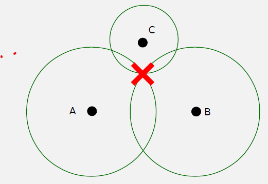
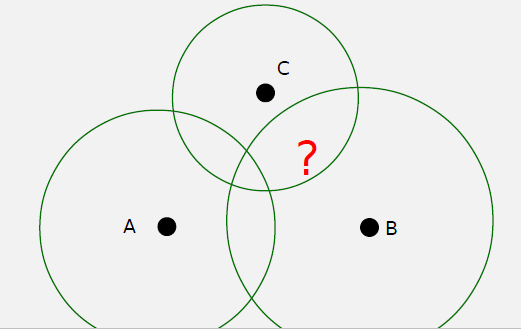
1505.6 Time Difference of Arrival (TDoA)
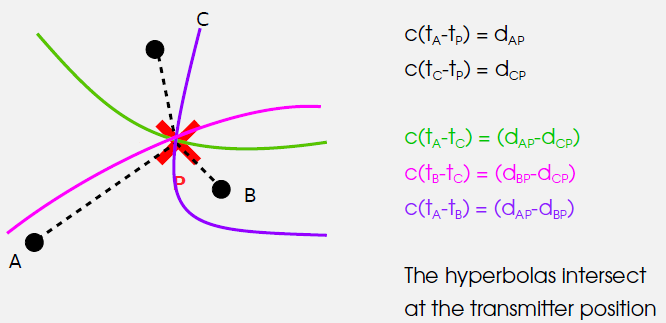
The Problem with Simple ToF: - Mobile device and fixed sites separated by large distances - Cannot keep clocks synchronized - RF signals travel at c, so 1 μs sync error = 300m position error
TDoA Solution: - Accept that clocks aren’t synced - Solve for the clock offset as an additional unknown - Any single range is wrong, but every range is wrong by the same amount - These erroneous ranges are called pseudoranges
%% fig-cap: "Time Difference of Arrival (TDoA) Positioning System"
%% fig-alt: "Diagram showing TDoA positioning system architecture with synchronized base stations"

%%{init: {'theme': 'base', 'themeVariables': { 'primaryColor': '#2C3E50', 'primaryTextColor': '#fff', 'primaryBorderColor': '#16A085', 'lineColor': '#16A085', 'secondaryColor': '#E67E22', 'tertiaryColor': '#ecf0f1', 'noteTextColor': '#2C3E50', 'noteBkgColor': '#fff3cd', 'textColor': '#2C3E50', 'fontSize': '16px'}}}%%

graph TB
    Mobile[Mobile Device<br/>Unsynchronized Clock<br/>Clock offset = unknown]

    Mobile -->|Signal| BS1[Base Station 1<br/>Synchronized<br/>Receives at T1]
    Mobile -->|Signal| BS2[Base Station 2<br/>Synchronized<br/>Receives at T2]
    Mobile -->|Signal| BS3[Base Station 3<br/>Synchronized<br/>Receives at T3]
    Mobile -->|Signal| BS4[Base Station 4<br/>Synchronized<br/>Receives at T4]

    BS1 --> Calc[TDoA Calculation]
    BS2 --> Calc
    BS3 --> Calc
    BS4 --> Calc

    Calc --> TD1[Time Difference:<br/>T2 - T1 = ΔT12]
    Calc --> TD2[Time Difference:<br/>T3 - T1 = ΔT13]
    Calc --> TD3[Time Difference:<br/>T4 - T1 = ΔT14]

    TD1 --> Position[Position Calculation<br/>4 unknowns:<br/>x, y, z, clock offset<br/>Need 4+ base stations]

    TD2 --> Position
    TD3 --> Position

    subgraph Key["Key Advantage"]
        Adv[Mobile clock can be wrong!<br/>Offset solved as unknown<br/>Pseudoranges all wrong<br/>by same amount]
    end

    style Mobile fill:#E67E22,stroke:#16A085,stroke-width:3px,color:#fff
    style BS1 fill:#2C3E50,stroke:#16A085,stroke-width:2px,color:#fff
    style BS2 fill:#2C3E50,stroke:#16A085,stroke-width:2px,color:#fff
    style BS3 fill:#2C3E50,stroke:#16A085,stroke-width:2px,color:#fff
    style BS4 fill:#2C3E50,stroke:#16A085,stroke-width:2px,color:#fff
    style Calc fill:#16A085,stroke:#2C3E50,stroke-width:3px,color:#fff
    style Position fill:#2C3E50,stroke:#16A085,stroke-width:3px,color:#fff
    style Adv fill:#E67E22,stroke:#16A085,stroke-width:3px,color:#fff
Key Requirements for TDoA:
- Base Stations Must Be Synchronized:
- Lay cables between stations
- Use GPS (ironically!)
- Give them all atomic clocks ($$$)
- Mobile Device Clock Can Be Wrong:
- Clock offset becomes an additional unknown to solve
- Need N+1 stations for N-dimensional positioning
- 3D position + clock offset = 4 unknowns → need 4 satellites
1505.7 GPS Architecture
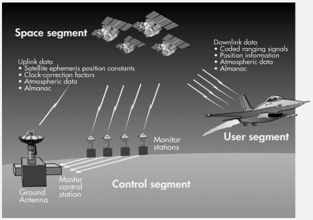
%% fig-cap: "GPS System Architecture - Three Segments"
%% fig-alt: "Complete GPS system architecture showing three interconnected segments"

%%{init: {'theme': 'base', 'themeVariables': { 'primaryColor': '#2C3E50', 'primaryTextColor': '#fff', 'primaryBorderColor': '#16A085', 'lineColor': '#16A085', 'secondaryColor': '#E67E22', 'tertiaryColor': '#ecf0f1', 'noteTextColor': '#2C3E50', 'noteBkgColor': '#fff3cd', 'textColor': '#2C3E50', 'fontSize': '16px'}}}%%

graph TB
    subgraph Space["Space Segment"]
        S1[31 GPS Satellites<br/>6 orbital planes<br/>MEO: 20,200 km]
        S2[Atomic Clocks<br/>Caesium/Rubidium<br/>±1 ns/day accuracy]
        S3[Signal Transmission<br/>L1: 1575 MHz<br/>L2: 1227 MHz<br/>L5: 1176 MHz]
    end

    subgraph Control["Control Segment"]
        C1[Master Control Station<br/>Schriever AFB, Colorado]
        C2[Monitor Stations<br/>Worldwide tracking]
        C3[Upload ephemeris<br/>Clock corrections<br/>Orbit adjustments]
    end

    subgraph User["User Segment"]
        U1[GPS Receivers<br/>Smartphones, vehicles<br/>IoT devices, drones]
        U2[Position Calculation<br/>Trilateration from<br/>4+ satellites]
        U3[Applications<br/>Navigation, tracking<br/>timing, surveying]
    end

    S1 -->|Broadcast signals| U1
    S3 -->|L1/L2/L5 signals| U1
    C2 -->|Monitor orbits<br/>Clock drift| C1
    C1 -->|Upload corrections| S1
    C3 -->|Ephemeris data| S1
    U1 --> U2
    U2 --> U3

    style S1 fill:#2C3E50,stroke:#16A085,stroke-width:3px,color:#fff
    style C1 fill:#16A085,stroke:#2C3E50,stroke-width:3px,color:#fff
    style U1 fill:#E67E22,stroke:#16A085,stroke-width:3px,color:#fff
    style U2 fill:#2C3E50,stroke:#16A085,stroke-width:2px,color:#fff
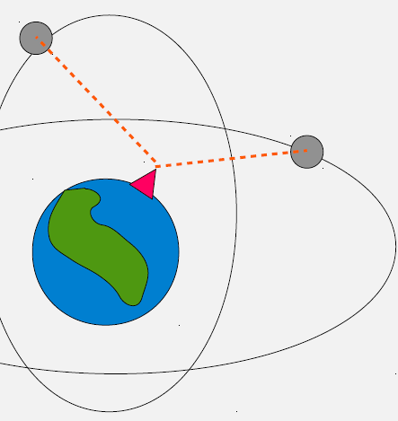
GPS is TDoA (Inverted):
- Satellites play the part of static devices (but are transmitters)
- Mobile device measures reception time using its clock
- Uses satellite’s transmitted time for the time difference
- For each satellite: measures (ToF + c × clockOffset)
- These are pseudoranges (erroneous distances)
1505.8 Satellite Synchronization
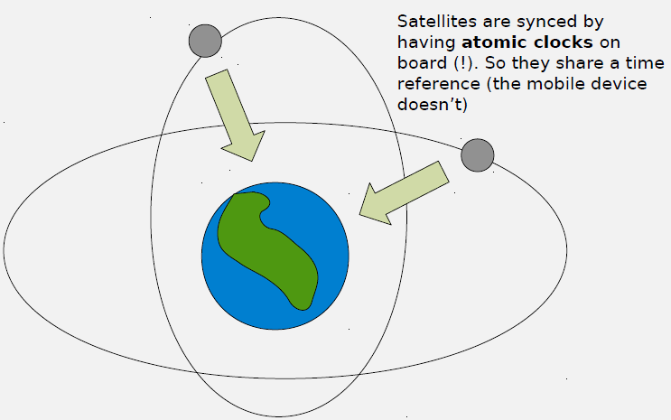
How Satellites Stay Synchronized:
- Atomic Clocks On Board (Caesium or Rubidium)
- Cost: ~$100,000 per clock
- Accuracy: ~1 nanosecond per day
- All satellites share time reference
- But They Aren’t Static?
- True! But we know their orbits precisely
- Can predict positions quite accurately
- Small errors do creep in…
- Ground Control Segment:
- Dedicated ground stations monitor satellite orbits
- Track actual positions vs predicted
- Upload corrections to satellites
- Must model relativistic effects!
Relativistic Effects: - Special Relativity: Satellite clocks run slower due to velocity (~7 μs/day slower) - General Relativity: Satellite clocks run faster due to weaker gravity (~45 μs/day faster) - Net Effect: ~38 μs/day faster → must be corrected!
1505.9 GPS Position Calculation
%% fig-cap: "GPS Position Calculation Process"
%% fig-alt: "Flowchart showing GPS position calculation from pseudoranges to final position"

%%{init: {'theme': 'base', 'themeVariables': { 'primaryColor': '#2C3E50', 'primaryTextColor': '#fff', 'primaryBorderColor': '#16A085', 'lineColor': '#16A085', 'secondaryColor': '#E67E22', 'tertiaryColor': '#ecf0f1', 'noteTextColor': '#2C3E50', 'noteBkgColor': '#fff3cd', 'textColor': '#2C3E50', 'fontSize': '16px'}}}%%

graph TB
    Start[GPS Receiver]

    Start --> Measure[Measure Pseudoranges<br/>ρ1, ρ2, ρ3, ρ4<br/>to 4+ satellites]

    Measure --> Ephemeris[Get Satellite Positions<br/>x1,y1,z1 ... x4,y4,z4<br/>from ephemeris data]

    Ephemeris --> Equations[4 Equations<br/>4 Unknowns]

    subgraph Unknowns["4 Unknowns to Solve"]
        U1[xr - receiver X]
        U2[yr - receiver Y]
        U3[zr - receiver Z]
        U4[Δt - clock offset]
    end

    Equations --> Solve[Solve Simultaneous<br/>Equations<br/>Iterative algorithm]

    Solve --> Correct[Apply Corrections<br/>Ionospheric delay<br/>Tropospheric delay<br/>Satellite clock errors]

    Correct --> Position[Final Position<br/>Latitude, Longitude<br/>Altitude<br/>±5-10m accuracy]

    subgraph Formula["Pseudorange Formula"]
        F[ρi = √x-xi² + y-yi² + z-zi² + c·Δt]
    end

    style Start fill:#2C3E50,stroke:#16A085,stroke-width:3px,color:#fff
    style Equations fill:#E67E22,stroke:#16A085,stroke-width:3px,color:#fff
    style Solve fill:#16A085,stroke:#2C3E50,stroke-width:3px,color:#fff
    style Position fill:#2C3E50,stroke:#16A085,stroke-width:3px,color:#fff
    style Formula fill:#E67E22,stroke:#16A085,stroke-width:2px,color:#fff
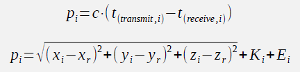
Position Equations:
For each satellite \(i\):
\[ \rho_i = \sqrt{(x_i - x_r)^2 + (y_i - y_r)^2 + (z_i - z_r)^2} + c \cdot \Delta t + E_i \]
Where: - \(\rho_i\) = pseudorange to satellite \(i\) (measured) - \((x_i, y_i, z_i)\) = satellite \(i\) position (known from ephemeris) - \((x_r, y_r, z_r)\) = receiver position (unknown) - \(c\) = speed of light - \(\Delta t\) = receiver clock offset (unknown) - \(E_i\) = error term (atmospheric delays, etc.)
Four Unknowns: 1. \(x_r\) (receiver X position) 2. \(y_r\) (receiver Y position) 3. \(z_r\) (receiver Z position) 4. \(\Delta t\) (clock offset)
Need at least 4 satellites to solve for 4 unknowns!
1505.10 GPS Error Sources
Signal Strength Challenge: - GPS signal transmitted at 20 watts - Travels 12,500 miles (20,000 km) - Received power: ~10^-16 watts (incredibly weak!) - Various atmospheric effects introduce errors
%% fig-cap: "GPS Error Sources and Magnitudes"
%% fig-alt: "Comprehensive breakdown of GPS error sources with typical magnitudes and mitigations"

%%{init: {'theme': 'base', 'themeVariables': { 'primaryColor': '#2C3E50', 'primaryTextColor': '#fff', 'primaryBorderColor': '#16A085', 'lineColor': '#16A085', 'secondaryColor': '#E67E22', 'tertiaryColor': '#ecf0f1', 'noteTextColor': '#2C3E50', 'noteBkgColor': '#fff3cd', 'textColor': '#2C3E50', 'fontSize': '16px'}}}%%

graph TB
    GPS[GPS Position<br/>Calculation]

    GPS --> Errors{Error Sources}

    Errors --> Ion[Ionospheric Delay<br/>±5 meters<br/>Refraction in<br/>ionosphere]
    Errors --> Trop[Tropospheric Delay<br/>±0.5 meters<br/>Water vapor,<br/>temperature]
    Errors --> Clock[Satellite Clock<br/>±2 meters<br/>Atomic clock drift]
    Errors --> Eph[Ephemeris Error<br/>±2.5 meters<br/>Orbit prediction<br/>inaccuracy]
    Errors --> Multi[Multipath<br/>±1 meter<br/>Signal reflections]
    Errors --> Noise[Receiver Noise<br/>±0.3 meters<br/>Electronics,<br/>antenna quality]

    Ion --> Mit1[Mitigation:<br/>Dual-frequency<br/>receivers]
    Trop --> Mit2[Mitigation:<br/>Atmospheric<br/>modeling]
    Clock --> Mit3[Mitigation:<br/>Ground station<br/>corrections]
    Eph --> Mit4[Mitigation:<br/>Frequent ephemeris<br/>updates]
    Multi --> Mit5[Mitigation:<br/>Antenna design,<br/>signal averaging]
    Noise --> Mit6[Mitigation:<br/>Better receivers,<br/>filtering]

    Mit1 --> Total[Total Error<br/>5-10 meters<br/>civilian GPS]
    Mit2 --> Total
    Mit3 --> Total
    Mit4 --> Total
    Mit5 --> Total
    Mit6 --> Total

    style GPS fill:#2C3E50,stroke:#16A085,stroke-width:3px,color:#fff
    style Errors fill:#E67E22,stroke:#16A085,stroke-width:3px,color:#fff
    style Ion fill:#E67E22,stroke:#16A085,stroke-width:2px,color:#fff
    style Trop fill:#E67E22,stroke:#16A085,stroke-width:2px,color:#fff
    style Clock fill:#E67E22,stroke:#16A085,stroke-width:2px,color:#fff
    style Eph fill:#E67E22,stroke:#16A085,stroke-width:2px,color:#fff
    style Multi fill:#E67E22,stroke:#16A085,stroke-width:2px,color:#fff
    style Noise fill:#E67E22,stroke:#16A085,stroke-width:2px,color:#fff
    style Total fill:#16A085,stroke:#2C3E50,stroke-width:3px,color:#fff
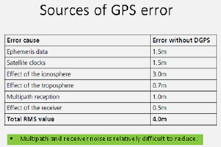
| Error Source | Typical Error | Mitigation |
|---|---|---|
| Ionospheric delay | ±5 m | Dual-frequency correction |
| Tropospheric delay | ±0.5 m | Modeling |
| Satellite clock | ±2 m | Ground station corrections |
| Ephemeris | ±2.5 m | Frequent updates |
| Multipath | ±1 m | Antenna design, averaging |
| Receiver noise | ±0.3 m | Better receivers |
1505.11 Knowledge Check
1505.12 What’s Next
Continue to GPS Accuracy and Enhancement to learn about the GPS error budget, differential GPS corrections, and RTK techniques that achieve centimeter-level accuracy for precision applications.