1628  Accelerometer Specification Case Study

1628.1 Learning Objectives

By the end of this chapter, you will be able to:

  • Analyze real-world datasheets: Walk through all sections of an accelerometer specification sheet
  • Interpret electrical specifications: Understand voltage, current, and ratiometric output calculations
  • Read performance metrics: Evaluate sensitivity, noise density, and bandwidth specifications
  • Understand mechanical specifications: Package dimensions, pin configurations, and mounting requirements
  • Apply timing and temperature specs: Account for startup time and temperature drift in designs

1628.2 Prerequisites

Before diving into this chapter, you should be familiar with:

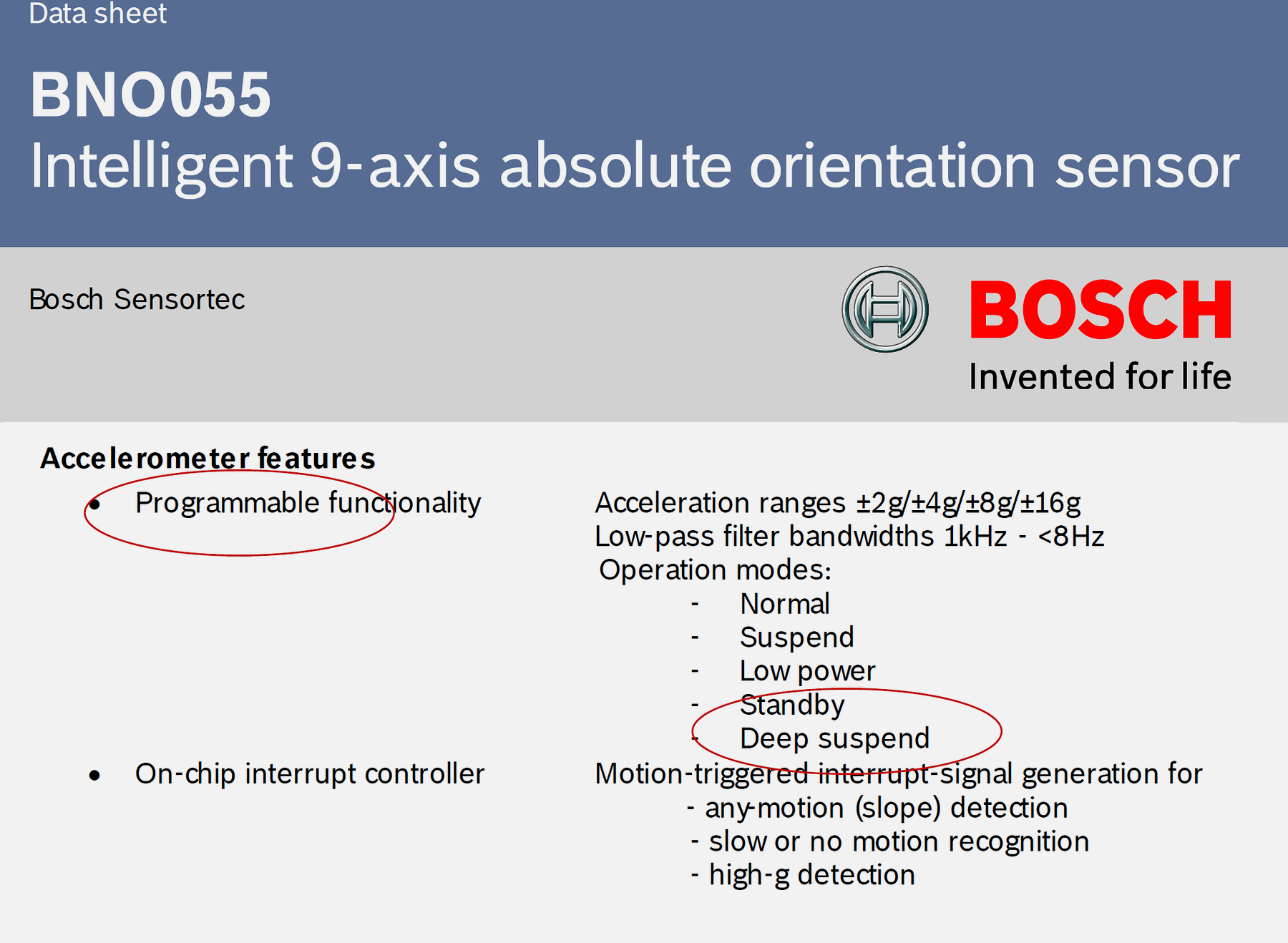
1628.3 Case Study: Accelerometer Specification Sheet

Let’s examine a real-world example: the +/-2g Tri-axis Analog Accelerometer specification sheet.

1628.3.1 Product Description

Accelerometer product overview page from datasheet showing device description, key features, and applications for the tri-axis analog accelerometer
Figure 1628.1: Product Overview

Key Information:

  • Product Name: Tri-axis Analog Accelerometer
  • Measurement Range: +/-2g (where g = 9.81 m/s^2)
  • Output Type: Analog voltage (ratiometric to supply voltage)
  • Axes: X, Y, Z (three-dimensional acceleration measurement)

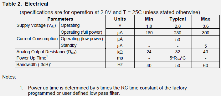
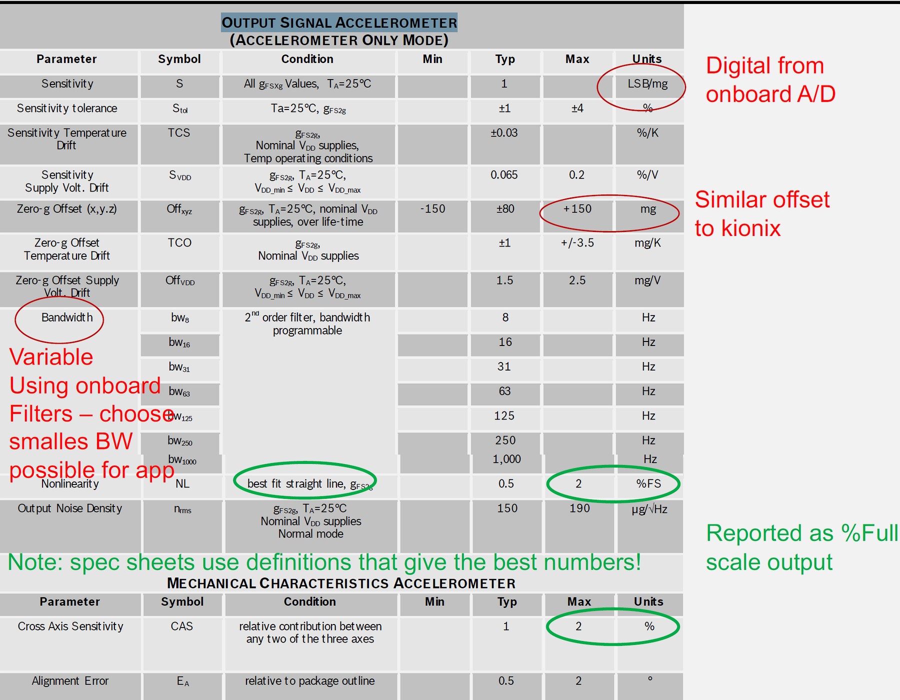
1628.3.2 Electrical Characteristics

Electrical specifications table from accelerometer datasheet showing supply voltage, current consumption, output voltage ranges, and sensitivity parameters
Figure 1628.2: Electrical Specifications

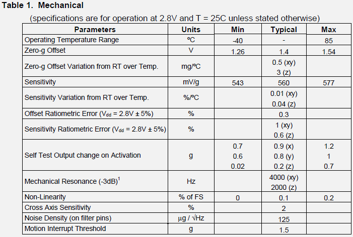
Critical Parameters:

Parameter Value Meaning
Supply Voltage (Vdd) 2.2V - 3.6V Operating voltage range
Supply Current 350 uA (typical) Current consumption during operation
Output Voltage Vdd/2 +/- sensitivity x acceleration Centered at half supply voltage
Sensitivity 800 mV/g (typical @ 3.0V) Output change per g of acceleration

Example Calculation:

If Vdd = 3.0V and measuring +1g on X-axis:
Vout_x = (3.0V / 2) + (0.8 V/g x 1g)
       = 1.5V + 0.8V
       = 2.3V

1628.3.3 Performance Specifications

Performance characteristics section showing measurement range, sensitivity, noise density, bandwidth, and other key performance metrics for the accelerometer
Figure 1628.3: Performance Characteristics

Key Performance Metrics:

  1. Measurement Range: +/-2g
    • Maximum measurable acceleration: 2 x 9.81 m/s^2 = 19.62 m/s^2
    • Suitable for: Human motion, orientation sensing, gentle impacts
  2. Sensitivity: 800 mV/g @ Vdd = 3.0V
    • Higher sensitivity = better resolution for small accelerations
    • Lower range devices typically have higher sensitivity
  3. Noise Density: ~150 ug/sqrt(Hz)
    • Lower noise = better precision
    • Impacts minimum detectable acceleration
  4. Bandwidth: 1600 Hz (typical)
    • Maximum frequency of acceleration changes that can be measured
    • Important for vibration monitoring, impact detection

1628.3.4 Mechanical Specifications

Mechanical specifications showing package dimensions, pin layout diagram, and physical mounting information for the LGA-16 package accelerometer
Figure 1628.4: Mechanical Characteristics

Package Information:

  • Package Type: LGA-16 (Land Grid Array, 16 pins)
  • Dimensions: 3mm x 3mm x 1mm
  • Weight: ~50 mg
  • Mounting: Surface mount (SMD)

Axis Orientation:

  • X, Y, Z axes clearly marked on package
  • Important for correct installation and interpretation

1628.3.5 Timing Diagrams

Timing diagram and specifications showing power-up sequence, turn-on time, and output response timing for the accelerometer
Figure 1628.5: Timing Specifications

Start-up and Response:

  • Turn-on Time: Time from power-up to valid output (~2ms typical)
  • Response Time: How quickly output changes with acceleration
  • Important for applications requiring fast response (e.g., airbag deployment)

1628.3.6 Temperature Characteristics

Temperature characteristics showing operating temperature range, sensitivity temperature coefficient, and zero-g offset temperature drift specifications
Figure 1628.6: Temperature Specs

Temperature Dependency:

  • Operating Range: -40C to +85C
  • Sensitivity Temperature Coefficient: +/-0.02% / C
  • Zero-g Offset Temperature Coefficient: +/-0.5 mg / C

Impact on Design:

Temperature change: 25C to 85C = 60C difference
Zero-g offset drift: 60C x 0.5 mg/C = 30 mg error

1628.3.7 Application Circuit

Recommended application circuit schematic showing decoupling capacitors, power connections, and output signal conditioning for the accelerometer
Figure 1628.7: Application Circuit

Supporting Components:

  • Decoupling Capacitors: 0.1uF near Vdd pin (noise filtering)
  • Output Capacitors: Optional filtering on outputs
  • Pull-up/Pull-down: Depending on interface requirements

1628.3.8 Pin Configuration

Pin configuration diagram showing the LGA-16 package pinout with Vdd, GND, X/Y/Z outputs, self-test pin, and NC pins labeled
Figure 1628.8: Pin Layout

Pin Functions:

  • Vdd: Power supply input
  • GND: Ground reference
  • X_OUT, Y_OUT, Z_OUT: Analog acceleration outputs
  • ST: Self-test pin (applies internal force to verify operation)
  • NC: No connection

1628.3.9 Ordering Information

Ordering information table showing part number variations for different ranges, interfaces, and package options
Figure 1628.9: Ordering Info

Part Number Variations:

  • Different ranges: +/-2g, +/-4g, +/-8g, +/-16g
  • Different interfaces: Analog, I2C, SPI
  • Different packages: LGA, QFN, DIP

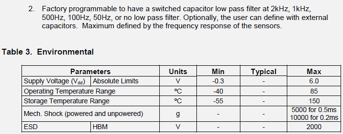
1628.3.10 Recommended Operating Conditions

Recommended operating conditions and absolute maximum ratings including supply voltage limits, storage temperature range, and ESD sensitivity specifications
Figure 1628.10: Operating Conditions

Critical Operating Parameters:

  • Supply Voltage Range: 2.2V - 3.6V (absolute max: -0.3V to 4.0V)
  • Storage Temperature: -40C to +125C
  • ESD Sensitivity: 2kV HBM (Human Body Model)

1628.4 Key Specification Parameters

Mind map diagram

Mind map diagram
Figure 1628.11: Mind map showing five critical specification categories in datasheets: electrical parameters including supply voltage and current consumption, performance metrics covering measurement capabilities and accuracy, timing characteristics defining response and sampling rates, mechanical specifications for physical integration, and environmental limits for operating and storage conditions essential for reliable IoT sensor deployment.

This flow variant shows which datasheet sections to focus on at different phases of your IoT project, from initial feasibility through production.

%% fig-cap: "Datasheet Reading Priority by Project Phase"
%% fig-alt: "Timeline showing which datasheet sections matter most at each project phase. Feasibility phase focuses on electrical specs (voltage, current) and key performance specs to validate concept. Prototyping phase adds timing diagrams, pinouts, and application circuits. Integration phase emphasizes interface details, register maps, and programming examples. Production phase focuses on absolute max ratings, quality grades, and reliability data. Each phase builds on previous knowledge."

%%{init: {'theme': 'base', 'themeVariables': { 'primaryColor': '#2C3E50', 'primaryTextColor': '#fff', 'primaryBorderColor': '#16A085', 'lineColor': '#16A085', 'secondaryColor': '#E67E22', 'tertiaryColor': '#fff', 'fontSize': '11px'}}}%%
graph TB
    subgraph Phase1["1. FEASIBILITY"]
        F1["Electrical: Voltage, Current"]
        F2["Performance: Range, Accuracy"]
        F3["Cost & Availability"]
    end

    subgraph Phase2["2. PROTOTYPING"]
        P1["Pinout & Package"]
        P2["Application Circuits"]
        P3["Timing Diagrams"]
    end

    subgraph Phase3["3. INTEGRATION"]
        I1["Register Maps"]
        I2["Communication Protocols"]
        I3["Code Examples"]
    end

    subgraph Phase4["4. PRODUCTION"]
        PR1["Absolute Max Ratings"]
        PR2["Quality & Reliability"]
        PR3["Ordering Information"]
    end

    Phase1 --> Phase2 --> Phase3 --> Phase4

    style F1 fill:#16A085,stroke:#2C3E50,color:#fff
    style F2 fill:#16A085,stroke:#2C3E50,color:#fff
    style P1 fill:#2C3E50,stroke:#16A085,color:#fff
    style P2 fill:#2C3E50,stroke:#16A085,color:#fff
    style I1 fill:#E67E22,stroke:#2C3E50,color:#fff
    style I2 fill:#E67E22,stroke:#2C3E50,color:#fff
    style PR1 fill:#7F8C8D,stroke:#2C3E50,color:#fff
    style PR2 fill:#7F8C8D,stroke:#2C3E50,color:#fff

Figure 1628.12: Different datasheet sections matter most at different project phases - don’t read the whole datasheet upfront, focus on what you need for your current phase.

1628.4.1 Understanding Measurement Range

Range Selection Criteria:

Graph diagram

Graph diagram
Figure 1628.13: Sensor measurement range selection decision tree showing trade-off between sensitivity and range for accelerometers: small range sensors like plus-minus 2g offer 800mV per g high sensitivity ideal for gentle motion detection, while large range plus-minus 16g sensors provide 100mV per g lower sensitivity suitable for impact and vibration monitoring applications.

Trade-off Relationship:

Larger Range -> Lower Sensitivity -> Lower Resolution
Smaller Range -> Higher Sensitivity -> Higher Resolution

1628.4.2 Understanding Accuracy vs Precision

Graph diagram

Graph diagram
Figure 1628.14: Visual comparison of accuracy versus precision using target analogy with four scenarios: high accuracy high precision shows tight cluster at target center representing ideal sensor performance, low accuracy high precision shows tight cluster offset from target indicating systematic calibration error, high accuracy low precision shows scattered readings around target indicating random noise, and low accuracy low precision shows worst case with scattered offset readings.

1628.5 Accelerometer Specification Visualizations

The following AI-generated diagrams provide enhanced visualizations of accelerometer specification concepts to supplement the datasheet analysis above.

Enhanced visualization of accelerometer key specifications showing measurement range as +/-2g spanning full vertical axis, sensitivity of 800mV/g as output slope, noise density as shaded uncertainty band, and bandwidth as frequency response curve up to 1600Hz.

Accelerometer Specification Overview
Figure 1628.15: Accelerometer specifications interact to define sensor performance. This visualization shows how range, sensitivity, noise, and bandwidth combine to determine the effective resolution and dynamic response for motion sensing applications.

Electrical specifications diagram showing supply voltage range from 2.2V to 3.6V, ratiometric output centered at Vdd/2, current consumption of 350 microamps, and power calculation for battery life estimation.

Accelerometer Electrical Characteristics
Figure 1628.16: Electrical characteristics determine integration requirements. This visualization explains how ratiometric output simplifies ADC reading (output scales with supply voltage), and how current consumption impacts battery life calculations.

Sensitivity diagram showing output voltage versus acceleration with 800mV/g slope, zero-g offset at Vdd/2, and how sensitivity determines resolution when paired with ADC bit depth and reference voltage.

Accelerometer Sensitivity Analysis
Figure 1628.17: Sensitivity determines measurement resolution. This visualization shows how 800mV/g sensitivity combined with a 12-bit ADC at 3.3V reference provides approximately 1mg resolution per LSB, enabling detection of small orientation changes.

Noise density visualization showing 150 microg per root Hz specification, integrated noise versus bandwidth calculation, and practical impact on minimum detectable acceleration for human activity recognition applications.

Accelerometer Noise Analysis
Figure 1628.18: Noise floor limits minimum detectable acceleration. This visualization demonstrates how noise density integrates with bandwidth to determine total RMS noise, and why reducing bandwidth through digital filtering improves effective resolution for slowly-varying signals like tilt measurement.

Frequency response diagram showing 1600Hz bandwidth as the minus 3dB point, anti-aliasing filter requirements when sampling at lower rates, and application examples for different bandwidth needs from tilt sensing to vibration analysis.

Accelerometer Bandwidth Considerations
Figure 1628.19: Bandwidth determines which motion frequencies are captured. This visualization maps bandwidth requirements to applications: orientation sensing needs only 10-50Hz, gesture recognition 50-200Hz, but vibration monitoring requires full 1600Hz bandwidth.

Package diagram showing LGA-16 footprint with dimensions, recommended PCB land pattern, axis orientation marked on package, and proper mounting alignment for consistent measurement direction across production.

Accelerometer Package and Mounting
Figure 1628.20: Package specifications ensure proper PCB integration. This visualization highlights the axis marking convention, recommended solder pad dimensions, and the importance of consistent orientation between design and production for reliable multi-axis measurements.

Temperature coefficient diagram showing sensitivity and offset drift across operating range from minus 40 to plus 85 degrees Celsius, with compensation techniques including factory calibration and runtime temperature correction.

Temperature Effects on Accelerometer
Figure 1628.21: Temperature affects both sensitivity and offset. This visualization shows how uncompensated accelerometer readings drift by 0.01%/C for sensitivity and 1mg/C for offset, requiring calibration or runtime compensation for precision applications.

Self-test mechanism diagram showing how internal electrostatic force deflects proof mass by known amount, expected output change in mV, and how self-test validates sensor functionality without physical motion for production testing.

Accelerometer Self-Test Feature
Figure 1628.22: Self-test enables production verification without motion. This visualization explains how the internal electrostatic actuator deflects the proof mass by a known amount, and how the expected output change confirms sensor functionality during manufacturing and field diagnostics.

Power mode comparison showing active mode at 350 microamps with full performance, low-power mode with reduced sampling rate at 100 microamps, and sleep mode at 3 microamps with motion interrupt wake capability.

Accelerometer Power Modes
Figure 1628.23: Power modes enable energy-efficient operation. This visualization compares current consumption across operating modes: full performance (350uA), low-power sampling (100uA), and sleep with motion wakeup (3uA), guiding duty cycle design for battery-powered applications.

Complete application schematic showing accelerometer with decoupling capacitors, analog output filtering, connection to microcontroller ADC pins, and optional interrupt pin routing for motion detection with component values annotated.

Accelerometer Application Circuit
Figure 1628.24: Application circuits translate datasheet specifications into working designs. This visualization shows recommended decoupling capacitors (0.1uF + 1uF), optional output filtering for noise reduction, and interrupt pin configuration for motion-triggered wakeup from low-power sleep.

1628.6 Summary

Key Takeaways from the Accelerometer Case Study:

  1. Electrical characteristics define power requirements and output behavior
    • Supply voltage range determines compatibility
    • Ratiometric output simplifies ADC integration
    • Current consumption impacts battery life
  2. Performance specifications determine measurement capability
    • Range and sensitivity trade-off (larger range = lower sensitivity)
    • Noise density limits minimum detectable signal
    • Bandwidth determines frequency response
  3. Mechanical specifications affect physical integration
    • Package type and dimensions for PCB layout
    • Axis orientation for correct measurement direction
    • Pin configuration for circuit design
  4. Temperature characteristics require compensation
    • Sensitivity and offset drift with temperature
    • Operating range must cover deployment environment
    • Factory or runtime calibration may be needed
  5. Application circuits show recommended implementation
    • Decoupling capacitors for noise filtering
    • Reference designs accelerate development

1628.7 What’s Next

Now that you understand how to read accelerometer datasheets in detail, continue to Sensor Selection Process to learn how to systematically compare multiple components and make optimal selection decisions for your IoT projects.

Related Chapters: