%%{init: {'theme': 'base', 'themeVariables': { 'primaryColor': '#2C3E50', 'primaryTextColor': '#fff', 'primaryBorderColor': '#16A085', 'lineColor': '#16A085', 'secondaryColor': '#E67E22', 'tertiaryColor': '#ECF0F1', 'fontFamily': 'Inter, system-ui, sans-serif'}}}%%
graph TD
    SOURCE["Source Code"] --> COMPILER{"Compiler<br/>Optimization"}

    COMPILER -->|"-O0"| O0["No Optimization<br/>Fast compile<br/>Easy debug<br/>Large/slow code"]
    COMPILER -->|"-O1/-O2"| O2["Balanced<br/>Moderate compile<br/>Good performance<br/>Reasonable size"]
    COMPILER -->|"-O3"| O3["Speed Focus<br/>Slow compile<br/>Aggressive inlining<br/>MASSIVE code size"]
    COMPILER -->|"-Os"| OS["Size Focus<br/>Moderate compile<br/>Compact code<br/>Reduced performance"]
    COMPILER -->|"-On"| ON["Custom Passes<br/>Fine control<br/>LLVM best<br/>Expert level"]

    style SOURCE fill:#E67E22,stroke:#2C3E50,stroke-width:2px,color:#fff
    style O0 fill:#E74C3C,stroke:#2C3E50,stroke-width:2px,color:#fff
    style O2 fill:#16A085,stroke:#2C3E50,stroke-width:2px,color:#fff
    style O3 fill:#F39C12,stroke:#2C3E50,stroke-width:2px,color:#fff
    style OS fill:#3498DB,stroke:#2C3E50,stroke-width:2px,color:#fff
    style ON fill:#9B59B6,stroke:#2C3E50,stroke-width:2px,color:#fff
1623 Software Optimization Techniques
1623.1 Learning Objectives
By the end of this chapter, you will be able to:
- Select appropriate compiler optimization flags: Choose between -O0, -O2, -O3, and -Os based on requirements
- Analyze code size considerations: Understand why flash memory dominates embedded system costs
- Apply SIMD vectorization: Exploit data-level parallelism for array processing
- Implement function inlining strategies: Balance call overhead against code size
- Design opportunistic sleeping patterns: Maximize battery life through intelligent power management
- Profile before optimizing: Use measurement to identify actual bottlenecks
1623.2 Prerequisites
Before diving into this chapter, you should be familiar with:
- Optimization Fundamentals: Understanding optimization trade-offs and priorities
- Hardware Optimization: Understanding the hardware capabilities that software optimization leverages
- Embedded Systems Programming: Familiarity with embedded C/C++ programming
1623.3 Software Optimisation
1623.3.1 Compiler Optimisation Choices
{fig-alt=“Compiler optimization level comparison showing trade-offs between -O0 (no optimization), -O1/-O2 (balanced), -O3 (speed-focused), -Os (size-focused), and -On (custom passes) in terms of compile time, code size, and performance”}
-O3 (Optimize for Speed): - May aggressively inline functions - Generates MASSIVE amounts of code - Re-orders instructions for better performance - Selects complex instruction encodings
-Os (Optimize for Size): - Penalizes inlining decisions - Generates shorter instruction encodings - Affects instruction scheduling - Fewer branches eliminated
-On (Custom Optimization): - Very specific optimization passes - Insert assembly language templates - LLVM is best for this
1623.3.2 Code Size Considerations
%%{init: {'theme': 'base', 'themeVariables': { 'primaryColor': '#2C3E50', 'primaryTextColor': '#fff', 'primaryBorderColor': '#16A085', 'lineColor': '#16A085', 'secondaryColor': '#E67E22', 'tertiaryColor': '#ECF0F1', 'fontFamily': 'Inter, system-ui, sans-serif'}}}%%
graph LR
    subgraph "Die Area Comparison @ 0.13um"
        M3["ARM Cortex M3<br/>0.43 mm2"]
        FLASH["128-Mbit Flash<br/>27.3 mm2"]
    end

    M3 -.->|"63x larger!"| FLASH

    subgraph "Code Size Strategies"
        DUAL["Dual Instruction Sets<br/>Thumb/Thumb-2<br/>16-bit + 32-bit"]
        CISC["CISC Encodings<br/>x86, System/360<br/>Complex instructions"]
        COMPRESS["Code Compression<br/>Decompress at runtime"]
    end

    FLASH --> DUAL
    FLASH --> CISC
    FLASH --> COMPRESS

    style M3 fill:#16A085,stroke:#2C3E50,stroke-width:2px,color:#fff
    style FLASH fill:#E74C3C,stroke:#2C3E50,stroke-width:3px,color:#fff
    style DUAL fill:#3498DB,stroke:#2C3E50,stroke-width:2px,color:#fff
    style CISC fill:#3498DB,stroke:#2C3E50,stroke-width:2px,color:#fff
    style COMPRESS fill:#3498DB,stroke:#2C3E50,stroke-width:2px,color:#fff
{fig-alt=“Code size impact diagram showing flash memory dominating die area (27.3mm2 vs 0.43mm2 for ARM Cortex M3) and three code size reduction strategies: dual instruction sets, CISC encodings, and code compression”}
Does code size matter? - 128-Mbit Flash = 27.3 mm2 @ 0.13um - ARM Cortex M3 = 0.43 mm2 @ 0.13um - Flash memory can dominate die area!
Dual Instruction Sets: Thumb/Thumb-2, ARCompact, microMIPS - 16-bit instructions have constraints (limited registers, reduced immediates)
CISC Instruction Sets: x86, System/360, PDP-11 - Complex encodings do more work - Require more complex hardware - Compiler support may be limited
1623.4 Advanced Software Optimizations
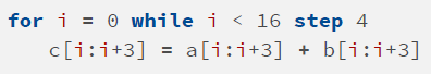
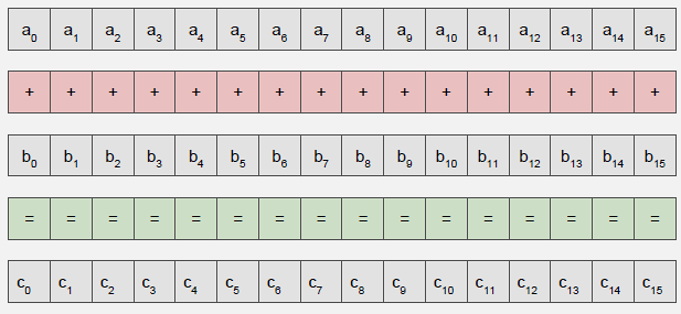
1623.4.1 Vectorization
%%{init: {'theme': 'base', 'themeVariables': { 'primaryColor': '#2C3E50', 'primaryTextColor': '#fff', 'primaryBorderColor': '#16A085', 'lineColor': '#16A085', 'secondaryColor': '#E67E22', 'tertiaryColor': '#ECF0F1', 'fontFamily': 'Inter, system-ui, sans-serif'}}}%%
sequenceDiagram
    participant Code as Source Code
    participant Scalar as Scalar Execution<br/>(1 element/instruction)
    participant SIMD as SIMD Vectorization<br/>(4 elements/instruction)

    Note over Code: for i = 0 to 999<br/>  array[i] = array[i] x 2

    rect rgb(231, 76, 60, 0.1)
        Note over Scalar: 1000 iterations
        loop 1000 times
            Scalar->>Scalar: Load 1 element
            Scalar->>Scalar: Multiply by 2
            Scalar->>Scalar: Store 1 element
        end
    end

    rect rgb(22, 160, 133, 0.1)
        Note over SIMD: 250 iterations (4x faster!)
        loop 250 times
            SIMD->>SIMD: Load 4 elements
            SIMD->>SIMD: Multiply 4x2 (parallel)
            SIMD->>SIMD: Store 4 elements
        end
    end

    Note over SIMD: Data-level parallelism<br/>Better memory bandwidth<br/>Fewer loop iterations
{fig-alt=“SIMD vectorization comparison showing scalar execution processing one element per iteration requiring 1000 iterations versus SIMD processing four elements per instruction requiring only 250 iterations for 4x speedup”}
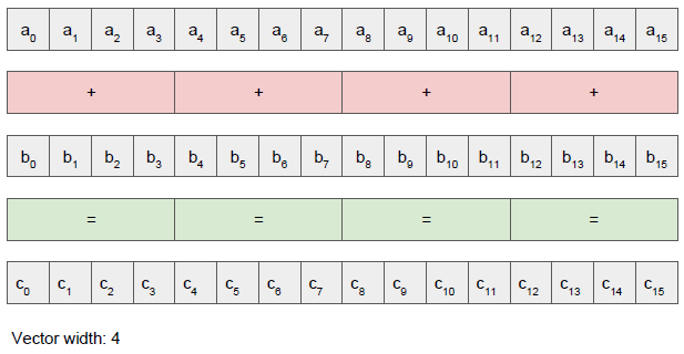
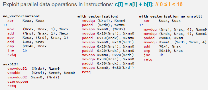
Key Idea: Operate on multiple data elements with single instruction (SIMD)
Benefits: - Fewer loop iterations - Better memory bandwidth utilization - Exploits data-level parallelism
Caution: Need extra code if vector width doesn’t divide iteration count exactly!


1623.4.2 Function Inlining
Advantages: - Low calling overhead - Avoids branch delay - Enables further optimizations
Limitations: - Not all functions can be inlined - Code size explosion possible - May require manual intervention (inline qualifier)
NoteFunction Inlining Trade-offs

Function inlining eliminates call overhead but increases code size, requiring careful analysis of which functions benefit from this optimization.
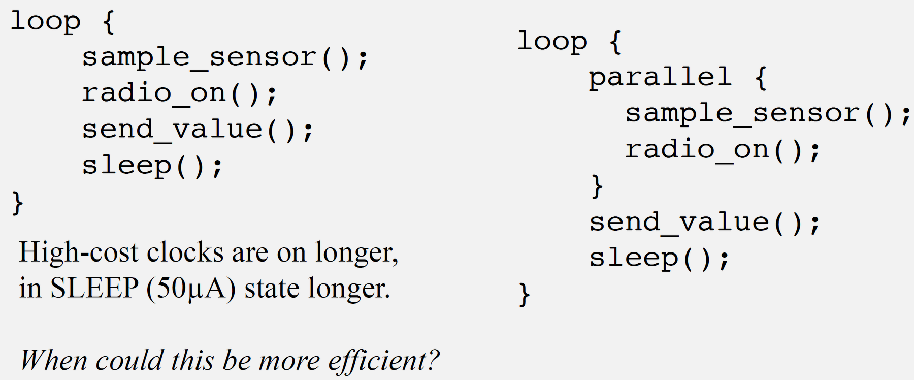
1623.4.3 Opportunistic Sleeping
Strategy: Transition processor and peripherals to lowest usable power mode ASAP
- Similar to stop/start in cars!
- Interrupts wake the processor for processing
- Balance energy savings vs reaction time


1623.5 Knowledge Check
CautionPitfall: Using printf/Serial.print for Timing-Critical Debug
The Mistake: Adding Serial.print() or printf() statements inside tight loops or ISRs to debug timing-sensitive code, then wondering why the bug disappears when debug output is added, or why the system becomes unreliable during debugging.
Why It Happens: Serial output is extremely slow compared to CPU operations. A single Serial.print("x") on Arduino at 115200 baud takes approximately 87 microseconds (10 bits per character at 115200 bps). In a 1 MHz loop (1 us per iteration), adding one print statement slows execution by 87x and changes all timing relationships. This creates “Heisenbugs” - bugs that disappear when you try to observe them.
The Fix: Use GPIO pin toggling for timing-critical debugging - set a pin HIGH at function entry, LOW at exit, and observe with an oscilloscope or logic analyzer. For capturing values without affecting timing, write to a circular buffer in RAM and dump after the critical section completes:
// WRONG: Serial output changes timing
void IRAM_ATTR timerISR() {
    Serial.println(micros());  // Takes 500+ us, destroys timing!
    processData();
}

// CORRECT: GPIO toggle for timing debug (oscilloscope required)
#define DEBUG_PIN 2
void IRAM_ATTR timerISR() {
    digitalWrite(DEBUG_PIN, HIGH);  // ~0.1 us
    processData();
    digitalWrite(DEBUG_PIN, LOW);   // ~0.1 us
}

// CORRECT: Buffer capture for value debug
volatile uint32_t debugBuffer[64];
volatile uint8_t debugIndex = 0;

void IRAM_ATTR timerISR() {
    if (debugIndex < 64) {
        debugBuffer[debugIndex++] = ADC_VALUE;  // ~0.2 us
    }
    processData();
}
// Dump buffer in loop() after critical operation completes
CautionPitfall: Optimizing Without Profiling (Premature Optimization)
The Mistake: Spending hours hand-optimizing a function that “looks slow” (like a nested loop or floating-point math) without measuring whether it actually impacts overall system performance, while ignoring the true bottleneck.
Why It Happens: Developers have intuitions about what should be slow based on algorithm complexity or “expensive” operations. But modern compilers optimize heavily, and I/O operations (network, storage, peripherals) often dominate execution time. A function with O(n^2) complexity processing 10 items (100 operations) may take 1 microsecond, while a single I2C sensor read takes 500 microseconds.
The Fix: Always profile before optimizing. On ESP32, use micros() to measure elapsed time. On ARM Cortex-M, use the DWT cycle counter (enabled via CoreDebug register). Identify the actual hotspot before optimizing:
// Step 1: Instrument code to find actual bottleneck
void loop() {
    uint32_t t0 = micros();
    readSensors();           // Suspect this is slow
    uint32_t t1 = micros();
    processData();           // Spent 2 weeks optimizing this
    uint32_t t2 = micros();
    transmitData();          // Never measured
    uint32_t t3 = micros();

    Serial.printf("Read: %lu us, Process: %lu us, Transmit: %lu us\n",
                  t1-t0, t2-t1, t3-t2);
}
// Typical result: Read: 2000 us, Process: 50 us, Transmit: 150000 us
// The "optimized" processData() was 0.03% of total time!
// Real fix: Reduce transmission frequency or payload size

// For ARM Cortex-M cycle-accurate profiling:
CoreDebug->DEMCR |= CoreDebug_DEMCR_TRCENA_Msk;  // Enable trace
DWT->CYCCNT = 0;                                   // Reset counter
DWT->CTRL |= DWT_CTRL_CYCCNTENA_Msk;              // Start counting
// ... code to measure ...
uint32_t cycles = DWT->CYCCNT;                    // Read cycles
Rule of thumb: 80% of execution time comes from 20% of code. Find the 20% first.

1623.6 Visual Reference Gallery
NoteVectorization Concepts
Source: CP IoT System Design Guide, Chapter 8 - Design and Prototyping
NoteScalar vs Vector Operations
Source: CP IoT System Design Guide, Chapter 8 - Design and Prototyping
NoteExploiting Parallelism
Source: CP IoT System Design Guide, Chapter 8 - Design and Prototyping
NoteLocal Computation vs Cloud
Source: CP IoT System Design Guide, Chapter 8 - Design and Prototyping
1623.7 Summary
Software optimization techniques are essential for efficient IoT firmware:
- Compiler Flags: -O3 for speed (large code), -Os for size (compact), -O2 for balance
- Code Size Matters: Flash memory dominates die area (27.3 mm2 vs 0.43 mm2 for CPU)
- Dual Instruction Sets: Thumb/Thumb-2 provide 30% code size reduction
- Vectorization (SIMD): Process 4+ elements per instruction for 4x+ speedup
- Function Inlining: Reduces call overhead but increases code size
- Opportunistic Sleeping: Transition to low-power modes ASAP
- Profile First: Measure actual bottlenecks before optimizing
The key is applying the right technique to the measured bottleneck, not optimizing based on assumptions.
1623.8 What’s Next
The next chapter covers Fixed-Point Arithmetic, which explores Qn.m format representation, conversion from floating-point, and efficient implementation on embedded processors without floating-point hardware.