215  Processes & Systems: PID Control

215.1 Learning Objectives

By the end of this chapter, you will be able to:

• Apply PID Control: Understand proportional, integral, and derivative control components
• Design Stable Systems: Evaluate trade-offs between different control strategies for IoT
• Tune PID Controllers: Find optimal gain values for system performance
• Implement Control Algorithms: Write PID control code for IoT devices
• Select Control Strategies: Choose appropriate methods based on system requirements

215.2 Prerequisites

Before diving into this chapter, you should be familiar with:

• Processes & Systems: Core Definitions: Understanding system decomposition and input-output transformations
• Processes & Systems: Control Types: Open-loop vs closed-loop control and feedback mechanisms
• Sensor Fundamentals and Types: How sensors measure physical phenomena for feedback
• Actuators: How actuators produce physical outputs in response to control signals

215.3 Getting Started (For Beginners)

TipWhat is PID Control? (Simple Explanation)

Analogy: PID control is like driving a car to a target speed:

• P (Proportional): The farther you are from target speed, the harder you press the gas
• I (Integral): If you’ve been slow for a while, press harder to catch up
• D (Derivative): If you’re approaching target fast, ease off to avoid overshooting

Combined: P + I + D = smooth, accurate approach to your target!

NoteKey Takeaway

In one sentence: PID combines three control actions—react to current error (P), eliminate persistent offset (I), and dampen oscillations (D)—to maintain precise setpoint control.

Remember this: Most real-world control systems (thermostats, drones, cruise control) use PID because it handles disturbances and changes automatically.

215.4 PID Control Basics for IoT

⭐⭐ Difficulty: Intermediate

Proportional-Integral-Derivative (PID) control is the most widely used feedback control algorithm in industrial automation and IoT systems. It combines three control actions to maintain a system at its desired setpoint.

TipKnowledge Check

Test your understanding of PID control concepts.

NoteQuiz 1: PID Controller Components

Question 1: A smart thermostat uses PID control to maintain room temperature at 22°C. The room is currently at 20°C and warming at 0.5°C per minute. Which PID term is MOST responsible for preventing the heater from overshooting past 22°C?

💡 Explanation: The Derivative (D) term responds to the rate of change of error. When temperature is rising at 0.5°C/min toward the 22°C setpoint, D detects this approach rate and starts reducing heater output before reaching the setpoint. This “predictive braking” prevents overshoot. The P term only reacts to current error (would keep heating until error=0). The I term accumulates error over time (actually increases overshoot risk). D is essential for high-inertia systems like HVAC where thermal mass causes continued temperature rise even after heater turns off.

InlineKnowledgeCheck = FileAttachment("/assets/js/iotclass-inline-knowledgecheck.js").text().then(text => {
  eval(text);
  return window.InlineKnowledgeCheck;
})

PID controller block diagram showing the three parallel control paths: Proportional, Integral, and Derivative

Figure 215.1: PID controller architecture: Three parallel control actions (Proportional, Integral, Derivative) combine to maintain setpoint accuracy while ensuring stability.

215.4.1 The PID Formula

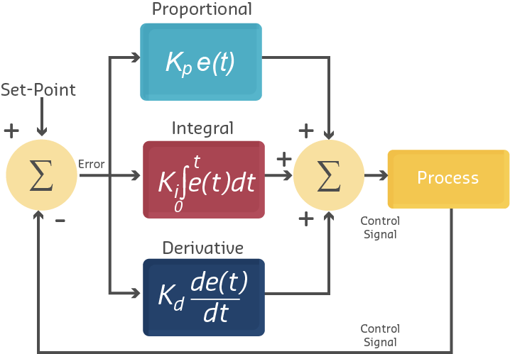
The PID controller calculates the control output \(u(t)\) based on the error \(e(t)\) between the setpoint and the measured value:

\[ u(t) = K_p \cdot e(t) + K_i \cdot \int_0^t e(\tau) \, d\tau + K_d \cdot \frac{de(t)}{dt} \]

Where: - \(u(t)\): Control output (e.g., valve position, motor speed, heater power) - \(e(t) = \text{setpoint} - \text{measured value}\): Current error - \(K_p\): Proportional gain (how strongly to react to current error) - \(K_i\): Integral gain (how strongly to correct accumulated past errors) - \(K_d\): Derivative gain (how strongly to react to error rate of change)

215.4.2 The Three Control Actions

1. Proportional (P) - React to Current Error:

• What it does: Output is proportional to the current error magnitude
• Effect: Larger error → stronger correction
• Problem: Never quite reaches setpoint (steady-state error)
• Analogy: Pushing harder on accelerator the farther you are from target speed

Example: Smart thermostat with P-only control: - Current temp: 18°C, Setpoint: 22°C → Error: 4°C - Control output: \(u = K_p \times 4\) (e.g., if \(K_p = 15\), then \(u = 60\%\) heater power) - As room warms to 21°C, error drops to 1°C → \(u = 15\%\) heater power - Problem: At 21.7°C, heater power equals heat loss → stuck below setpoint!

2. Integral (I) - Account for Accumulated Error:

• What it does: Accumulates error over time and corrects for persistent offset
• Effect: Eliminates steady-state error (eventually reaches exact setpoint)
• Problem: Can cause overshoot and slow oscillations if too aggressive
• Analogy: Remembering that you’ve been consistently behind schedule and compensating

Example: Adding I-control to thermostat: - Even when temp hovers at 21.7°C (error = 0.3°C), integral term keeps growing - \(\int e(t) dt\) accumulates: 0.3 + 0.3 + 0.3… over many time steps - Eventually integral term adds enough output to push temp to exactly 22°C - Benefit: Reaches exact setpoint, not just “close enough”

3. Derivative (D) - Predict Future Error:

• What it does: Responds to rate of change of error (how fast it’s changing)
• Effect: Dampens oscillations, improves stability, slows overshoot
• Problem: Amplifies sensor noise (small noise fluctuations look like large rate changes)
• Analogy: Seeing you’re approaching target speed quickly and easing off accelerator early

Example: Adding D-control to thermostat: - Temp rising rapidly from 18°C → 19°C → 20°C (1°C per minute) - \(de/dt = -1°C/\text{min}\) (error decreasing at 1°C/min) - D-term reduces output before reaching setpoint: “We’re getting there fast—slow down!” - Benefit: Less overshoot, smoother approach to setpoint

%%{init: {'theme': 'base', 'themeVariables': { 'primaryColor': '#2C3E50', 'primaryTextColor': '#fff', 'primaryBorderColor': '#16A085', 'lineColor': '#16A085', 'secondaryColor': '#E67E22', 'tertiaryColor': '#7F8C8D'}}}%%
sequenceDiagram
    participant SP as Setpoint<br/>22.0 C
    participant CTRL as PID Controller
    participant HVAC as HVAC System
    participant ROOM as Clean Room
    participant SENS as Temp Sensor

    Note over SP,SENS: t=0s: Initial state - Room at 20.0 C

    SP->>CTRL: Target: 22.0 C
    SENS->>CTRL: Measured: 20.0 C
    Note over CTRL: Error = +2.0 C<br/>P=70%, I accumulating, D=0

    CTRL->>HVAC: Output: 70% heating
    HVAC->>ROOM: Heat input HIGH

    Note over SP,SENS: t=60s: Room warming

    SENS->>CTRL: Measured: 21.2 C
    Note over CTRL: Error = +0.8 C<br/>P=28%, I growing, D negative

    CTRL->>HVAC: Output: 35% heating
    Note over CTRL: D-term reduces output<br/>anticipating approach

    Note over SP,SENS: t=120s: Near setpoint

    SENS->>CTRL: Measured: 21.9 C
    Note over CTRL: Error = +0.1 C<br/>P=3%, I eliminates offset, D braking

    CTRL->>HVAC: Output: 12% heating
    HVAC->>ROOM: Maintain steady state

    Note over SP,SENS: t=180s: Stable at 22.0 C +/- 0.08 C

Figure 215.2: Timeline sequence showing how PID control responds over time. Initial large error triggers strong P-term response, D-term anticipates approach to prevent overshoot, and I-term eliminates steady-state offset.

215.4.3 Tuning PID Controllers

Finding the right \(K_p\), \(K_i\), \(K_d\) values is critical:

Parameter	Too Low	Optimal	Too High
\(K_p\) (Proportional)	Slow response, large steady-state error	Fast response, minimal overshoot	Overshoot, oscillations, instability
\(K_i\) (Integral)	Persistent offset, never reaches setpoint	Eliminates offset, stable	Large overshoot, slow oscillations
\(K_d\) (Derivative)	Overshoot, oscillations	Smooth approach, damped response	Noise amplification, erratic behavior

Common Tuning Methods:

1. Ziegler-Nichols Method: Empirical tuning based on step response
2. Manual Tuning: Start with P-only, add I to eliminate offset, add D to reduce overshoot
3. Auto-Tuning: Modern controllers can self-tune by observing system response

InlineKnowledgeCheck({
  id: "mutex-vs-semaphore-use-cases",
  question: "An IoT weather station has: (1) Shared UART console for debug logging from 3 tasks, (2) Circular buffer (size=10) for sensor readings (producer tasks write, consumer task reads). Which synchronization primitives should be used?",
  options: [
    "UART: Binary semaphore (value 0/1); Buffer: Binary semaphore (value 0/1)",
    "UART: Mutex (ownership tracking); Buffer: Counting semaphore (value 0-10) + mutex",
    "UART: Counting semaphore (value 0-3); Buffer: Mutex (exclusive access)",
    "UART: Spin-lock (busy-waiting); Buffer: Binary semaphore (value 0/1)"
  ],
  correctIndex: 1,
  explanation: "**UART needs mutex**: (1) **Mutual exclusion**: Only one task can write to UART at a time—prevents garbled output. (2) **Ownership**: Mutex tracks which task holds it—enables priority inheritance (if high-priority task blocks on UART held by low-priority task, low-priority inherits high priority temporarily). (3) **Recursive locking**: If same task calls nested log functions, mutex allows reacquisition. **Buffer needs counting semaphore + mutex**: (1) **Counting semaphore** (0-10): Tracks available slots—producers block when full (count=0), consumers block when empty (count=0). (2) **Mutex**: Protects actual buffer manipulation—prevents two producers from writing to same index simultaneously. **Why binary semaphore insufficient**: Can't count slots (only signals full/empty binary state). **Why spin-lock fails**: Wastes CPU cycles—acceptable only for very short critical sections (microseconds) with interrupts disabled, not multi-millisecond I/O. **Real RTOS example**: `xSemaphoreCreateMutex()` for UART, `xSemaphoreCreateCounting(10, 10)` + `xSemaphoreCreateMutex()` for buffer.",
  difficulty: "Intermediate"
})

InlineKnowledgeCheck({
  id: "resource-allocation-strategies",
  question: "An IoT gateway with 512KB RAM runs dynamic memory allocation for sensor data packets (average 2KB, arrival rate varies 10-100/sec). The system experiences memory fragmentation causing allocation failures despite 150KB free memory shown. Which resource allocation strategy BEST addresses this?",
  options: [
    "First-fit allocation - allocate from first sufficiently large free block found, fastest allocation",
    "Best-fit allocation - allocate from smallest sufficient free block, minimizes wasted space per allocation",
    "Memory pool (fixed-size blocks) - pre-allocate array of 2KB blocks, no fragmentation",
    "Compacting garbage collector - periodically defragment memory by moving allocated blocks together"
  ],
  correctIndex: 2,
  explanation: "**Memory pool (Option C)** is optimal for embedded IoT: Pre-allocate **256 blocks of 2KB** (512KB total). Each `malloc()` returns pre-allocated block, `free()` returns to pool. **Advantages**: (1) **Zero fragmentation**: Fixed-size blocks prevent external fragmentation (gaps between allocations). (2) **Deterministic timing**: Allocation/free is O(1)—critical for real-time systems (first-fit/best-fit search takes variable time). (3) **No memory leaks**: Pool size is bounded—detect leaks when pool exhausted. (4) **Cache-friendly**: Contiguous block array improves cache locality. **Why first/best-fit fail**: Variable-size allocations cause fragmentation over time (150KB free but scattered in 500-byte chunks unusable for 2KB requests). **Why garbage collection fails**: (1) GC pause times (10-100ms) unacceptable for real-time IoT. (2) Requires language runtime (Java/Python)—adds 5-20MB overhead. (3) Embedded C/C++ lacks automatic GC. **Implementation**: Use **FreeRTOS memory pools** (`xQueueCreate()` for pool management) or custom pool: `uint8_t pool[256][2048]; bool used[256];`. **Real IoT example**: lwIP network stack uses memory pools (PBUF_POOL) for packet buffers.",
  difficulty: "Advanced"
})

215.5 Real IoT PID Control Examples

215.5.1 Example 1: Smart Thermostat (Temperature Control)

System Components:

Component	Details	IoT Integration
Setpoint	Desired temperature: 22°C	Set via smartphone app or voice assistant
Sensor	DHT22 temperature sensor (±0.5°C)	I2C interface to ESP32 microcontroller
Controller	PID algorithm (\(K_p=15\), \(K_i=0.5\), \(K_d=5\))	Runs every 30 seconds on ESP32
Actuator	Smart relay controlling HVAC system	240V relay switched by GPIO pin
Process	Room thermal dynamics (5-10 min time constant)	Cloud logging of temperature history

Operation:

1. Measure: Sensor reads 18.5°C
2. Error: 22.0 - 18.5 = 3.5°C
3. P-term: 15 × 3.5 = 52.5
4. I-term: 0.5 × Σ(errors) = 0.5 × 12.3 = 6.15 (accumulated over past 5 minutes)
5. D-term: 5 × (3.5 - 3.8)/30s = -0.05 (error decreasing slowly)
6. Output: 52.5 + 6.15 - 0.05 = 58.6% heater duty cycle
7. Actuate: HVAC runs at 58.6% power for next 30 seconds
8. Repeat: Measure again after 30 seconds

Results: - Settling Time: 8 minutes to reach 22°C ±0.2°C - Overshoot: <0.3°C (minimal temperature overshoot) - Energy Savings: 23% reduction vs simple on/off thermostat - Comfort: ±0.2°C stability vs ±1.5°C with on/off control

215.5.2 Example 2: Drone Stability (Orientation Control)

System Components:

Component	Details	Update Rate
Setpoint	Target orientation: level (0° pitch, 0° roll)	User joystick commands
Sensor	MPU-6050 IMU (gyroscope + accelerometer)	100 Hz (every 10ms)
Controller	Cascaded PID loops (angle PID → rate PID)	400 Hz (every 2.5ms)
Actuator	4× brushless motors with ESCs	PWM 1000-2000µs pulse width
Process	Quadcopter rotational dynamics	<50ms response time

Dual-Loop Control (Cascaded PID):

Outer Loop (Angle Control): - Setpoint: 0° pitch (level flight) - Measured: Accelerometer reads 5° nose-down pitch - Error: 0° - 5° = -5° - PID Output: Desired pitch rate = +30°/sec (rotate nose up)

Inner Loop (Rate Control): - Setpoint: +30°/sec (from outer loop) - Measured: Gyroscope reads +10°/sec (rotating up, but too slowly) - Error: +30°/sec - 10°/sec = +20°/sec - PID Output: Increase rear motors by 15%, decrease front motors by 15% - Result: Drone pitches nose up at 30°/sec → returns to level

Why Two Loops? - Outer loop (slow): Strategic goal—“Get to level orientation” - Inner loop (fast): Tactical execution—“Rotate at this exact rate” - Benefit: Faster response, better stability than single-loop control

215.5.3 Example 3: Water Tank Level Control

System Setup:

Component	Specification	Purpose
Setpoint	75% tank level	Maintain optimal water supply
Sensor	Ultrasonic distance sensor (HC-SR04, ±3mm)	Measure water level every 5 seconds
Controller	Arduino Uno running PID library	Calculate pump speed (0-100%)
Actuator	Variable speed pump (0-50 liters/min)	Controlled via PWM to motor driver
Process	1000-liter water tank (60cm × 60cm × 278cm)	5-minute time constant

Control Challenges:

1. Disturbances: Water consumption varies (0-30 L/min depending on household usage)
2. Nonlinearity: Pump efficiency changes with tank level (less efficient at low levels)
3. Noise: Ultrasonic sensor has ±3mm noise (~0.3% of tank height)

PID Solution (\(K_p=20\), \(K_i=0.8\), \(K_d=8\)):

Scenario: Heavy water usage (shower + dishwasher)
1. Tank drops: 75% → 70% → 65% in 2 minutes
2. Error grows: 10% below setpoint
3. P-term: 20 × 10 = 200 → pump at 100% (capped at max speed)
4. I-term accumulates: 0.8 × Σ(errors) = keeps pump running even as level recovers
5. D-term: Sees rapid level drop (de/dt large) → boosts pump early
6. Result: Tank refills to 75% in 8 minutes, stabilizes with ±1% fluctuation

Performance Metrics:

Metric	Without PID (On/Off Control)	With PID Control
Level Stability	±8% variation	±1% variation
Pump Starts/Hour	12 starts (wear and energy spikes)	2-3 starts (soft start via PWM)
Water Shortage Events	3 per month (tank empty)	0 per year
Energy Consumption	2.8 kWh/day (frequent on/off)	2.1 kWh/day (smooth operation)
Pump Lifespan	~3 years (mechanical stress)	~7 years (gentle operation)

InlineKnowledgeCheck({
  id: "rtos-concepts-tick-rate",
  question: "An IoT environmental monitor runs FreeRTOS with configTICK_RATE_HZ = 100 (10ms tick period). It has a task that must sample a vibration sensor every 3ms to detect machinery faults. The developer uses `vTaskDelay(3)` expecting 3ms delay. What is the actual behavior?",
  options: [
    "Task wakes every 3ms as expected - vTaskDelay() uses hardware timers independent of tick rate",
    "Task wakes every 30ms - vTaskDelay(3) means 3 ticks × 10ms/tick = 30ms actual delay",
    "Task wakes immediately - vTaskDelay() with value less than tick period returns instantly",
    "Compilation error - vTaskDelay() parameter must be multiple of configTICK_RATE_HZ"
  ],
  correctIndex: 1,
  explanation: "**vTaskDelay(3) means 3 TICKS, not 3 milliseconds**: With configTICK_RATE_HZ=100 (10ms/tick), `vTaskDelay(3)` = 3 ticks × 10ms = **30ms delay**. This is 10× slower than the required 3ms sampling! **Why this is critical**: Vibration analysis (FFT) requires consistent high-rate sampling (Nyquist theorem: sample at 2× highest frequency). Missing samples at 30ms (33 Hz) vs required 3ms (333 Hz) loses 90% of data, making fault detection impossible. **Solutions**: (1) **Increase tick rate**: Set configTICK_RATE_HZ=1000 (1ms/tick) → `vTaskDelay(3)` = 3ms. Trade-off: More frequent tick interrupts = higher overhead (0.2% → 2% CPU on context switching). (2) **Use hardware timer interrupt**: Configure timer to trigger ISR every 3ms, sample in ISR, signal task via semaphore. More efficient for sub-tick timing. (3) **Use high-resolution timer APIs**: Some RTOSes provide microsecond APIs (e.g., ESP-IDF `esp_timer_start_periodic()`). **Best practice**: Match tick rate to finest required timing resolution, use hardware timers for sub-tick timing.",
  difficulty: "Intermediate"
})

InlineKnowledgeCheck({
  id: "real-time-priority-ceiling-protocol",
  question: "An industrial IoT controller runs three tasks sharing two resources (SPI bus, SD card). **Task1** (Priority 10, highest): Emergency data logging (uses SPI+SD). **Task2** (Priority 5): Normal logging (uses SPI+SD). **Task3** (Priority 3): Status LED (no shared resources). To prevent priority inversion and unbounded blocking, which advanced RTOS protocol should be implemented?",
  options: [
    "Priority inheritance protocol (PIP) - task holding resource inherits priority of blocked high-priority task",
    "Priority ceiling protocol (PCP) - each resource has ceiling priority equal to highest priority of any task that uses it; task inherits ceiling when acquiring resource",
    "Immediate priority ceiling protocol (IPCP) - task immediately jumps to resource ceiling priority upon lock acquisition, even if no tasks are blocked",
    "No special protocol - careful coding with proper lock ordering is sufficient"
  ],
  correctIndex: 2,
  explanation: "**Immediate Priority Ceiling Protocol (IPCP)** is optimal for hard real-time systems: Assign **resource ceiling priorities**: SPI ceiling = 10 (Task1 uses it), SD ceiling = 10 (Task1 uses it). When Task2 (Priority 5) acquires SPI mutex, it **immediately** inherits Priority 10—even before Task1 blocks. **Why IPCP wins**: (1) **Prevents priority inversion**: Task2 runs at Priority 10 while holding SPI—Task3 (Priority 3) never preempts it mid-critical-section. (2) **Bounded blocking**: Task1 can be blocked at most once per resource—when Task1 tries to acquire SPI held by Task2, Task2 already runs at Priority 10 and finishes quickly. (3) **Deadlock-free**: No circular wait possible—task running at ceiling priority cannot be blocked by any task. **Why PIP is weaker**: Only inherits priority **after** high-priority task blocks—allows transitive blocking (Task3 runs before Task2 inherits priority, wastes time). **Why PCP differs from IPCP**: PCP inherits ceiling only when higher-priority task blocks; IPCP inherits immediately (more predictable, simpler analysis). **Real systems**: Safety-critical RTOS (RTEMS, VxWorks) implement IPCP for deterministic worst-case response time analysis (required for DO-178C avionics certification).",
  difficulty: "Advanced"
})

215.6 When to Use PID vs Simpler Control

Not every IoT system needs PID control. Here’s a decision framework:

Scenario	Control Strategy	Reasoning
Simple on/off (LED, valve)	Bang-bang (on/off) control	No proportional control needed—device is either on or off
Slow process, low precision (room temp ±2°C OK)	Simple thermostat (on when cold, off when hot)	Thermal inertia provides natural smoothing
Fast process, high precision (drone, motor)	PID required	Must respond quickly and accurately to avoid instability
Multiple interacting variables (HVAC: temp + humidity)	Multi-loop PID or advanced control	Single-variable PID insufficient for coupled systems
Highly nonlinear (battery charging)	Look-up table + PID trim	PID struggles with extreme nonlinearity—hybrid approach better
Safety-critical (medical, automotive)	PID + redundancy + fault detection	Reliability and failsafes essential

Rule of Thumb: - Bang-bang control: Simple, cheap, acceptable performance (±10% tolerance) - PID control: Moderate complexity, better performance (±1-2% tolerance) - Advanced control (MPC, adaptive): High complexity, optimal performance (<±0.5% tolerance)

IoT-Specific Considerations:

1. Computational Resources: PID requires floating-point math—ensure MCU can handle it at required sample rate
2. Sensor Quality: Noisy sensors → add filtering before PID or reduce derivative gain
3. Communication Latency: If control loop spans cloud (sensor → cloud → actuator), latency may prevent effective PID → use edge computing
4. Energy Constraints: Continuous PID sensing/actuation consumes power → consider duty-cycled control for battery devices

TipCross-Hub Connections

Interactive Learning Tools: - Simulations Hub - Try the PID Tuner Simulator to see how changing Kp, Ki, Kd affects system response - Videos Hub - Watch PID control demonstrations showing real controllers, tuning methods, and system stability - Quizzes Hub - Test your understanding of PID components, tuning, and control strategy selection

Knowledge Resources: - Knowledge Gaps Hub - Common misconceptions about PID tuning and stability explained - Knowledge Map - See how PID control connects to sensors, actuators, and system design

NoteRelated Chapters

This Series: - Processes & Systems: Core Definitions - What are processes and systems - Processes & Systems: Control Types - Open-loop vs closed-loop control

Deep Dives: - Process Control and PID - Advanced feedback control systems - Processes Labs and Review - Hands-on implementations - PID Feedback Fundamentals - Mathematical foundations

Foundation: - IoT Reference Models - System architecture layers - State Machines in IoT - Control state management

Sensing & Actuation: - Sensor Fundamentals - Input devices - Actuators - Output devices - Sensor Circuits - Interfacing

Design: - Energy Management - Power optimization - Hardware Prototyping - System building

215.7 Visual Reference Gallery

NoteVisual: Coffee Pot Control System Block Diagram

Block diagram of a coffee pot control system

This visualization illustrates the fundamental closed-loop control concepts using a familiar household appliance, demonstrating how sensors, controllers, and actuators work together.

NoteVisual: Closed-Loop Feedback System

Closed-loop feedback control system architecture

This diagram shows the general architecture of closed-loop feedback systems fundamental to understanding PID control and IoT process automation.

NoteVisual: Adding Integral Control Action

Adding integral control to eliminate steady-state error

This figure demonstrates how integral control eliminates steady-state error by integrating accumulated error over time, a key concept in PID controller design.

215.8 Summary

This chapter covered PID control theory and applications for IoT:

• PID Control Theory: Learning the three control actions—Proportional (react to current error), Integral (eliminate accumulated error), and Derivative (predict and dampen oscillations)
• The PID Formula: Understanding the mathematical relationship \(u(t) = K_p \cdot e(t) + K_i \cdot \int e(\tau) d\tau + K_d \cdot \frac{de}{dt}\)
• PID Tuning: Finding optimal gain values (\(K_p\), \(K_i\), \(K_d\)) to balance response speed, stability, and precision
• Real-World PID Applications: Implementing feedback control in smart thermostats (temperature regulation), drones (orientation stability), and water tanks (level control)
• Cascaded Control: Using dual PID loops for improved performance in fast systems like drones
• Control Strategy Selection: Choosing appropriate control methods based on system dynamics, precision requirements, computational resources, and energy constraints
• IoT-Specific Considerations: Addressing computational resources, sensor noise, communication latency, and energy constraints in control design

215.9 What’s Next

The next chapter explores State Machines in IoT, introducing how to manage system modes and transitions. You’ll learn how state machines complement PID control by managing higher-level system behavior (startup, shutdown, fault handling) while PID handles continuous regulation within each state.