214  Processes & Systems: Control Types

214.1 Learning Objectives

By the end of this chapter, you will be able to:

• Compare Control Types: Differentiate between open-loop and closed-loop control systems
• Analyze Feedback Loops: Describe how feedback mechanisms maintain system stability
• Understand System Stability: Evaluate trade-offs between different control strategies for IoT
• Implement Self-Regulation: Build systems that automatically adjust to maintain desired behavior
• Apply Control Concepts: Select appropriate control strategies for different IoT scenarios

214.2 Prerequisites

Before diving into this chapter, you should be familiar with:

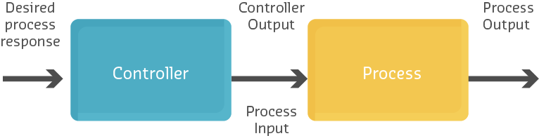
• Processes & Systems: Core Definitions: Understanding system decomposition and input-output transformations
• Sensor Fundamentals and Types: How sensors measure physical phenomena for feedback
• Actuators: How actuators produce physical outputs in response to control signals

214.3 Getting Started (For Beginners)

TipOpen-Loop vs Closed-Loop: The Core Concept

This is the most important concept in control systems:

Type	How It Works	Example	Problem
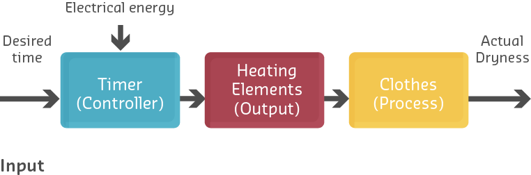
Open-Loop	Set it and forget it	Toaster with timer	Burns toast if bread is thick
Closed-Loop	Continuously adjusts based on feedback	Thermostat	More complex, more reliable

214.3.1 Real-World Comparison

Control System Comparison:

Type	Device	Command	Behavior	Result
OPEN-LOOP (Dumb)	Space Heater	“Run for 2 hours”	Runs regardless of temperature	Maybe too hot or cold!
CLOSED-LOOP (Smart)	Smart Thermostat	“Keep room at 22°C”	Checks actual temp and adjusts	Always comfortable!

214.3.2 Feedback Loop Explained

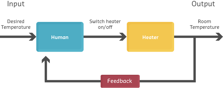
NoteThe Shower Temperature Problem

Everyone has experienced this control system:

Goal: Get water at perfect temperature (38°C)

Step	Component	Action
1	Desired Temp (Setpoint)	You want 38°C
2	Valve (Actuator)	Turn valve to adjust
3	Water Temp (Output)	Water comes out
4	Your Hand (Sensor)	Feel water temperature
5	Feedback Loop	Compare to desired → Adjust valve → Repeat!

This is a CLOSED-LOOP control system—you are the controller!

214.3.3 IoT Examples of Control Systems

Example 1: Smart Irrigation

Smart Irrigation Comparison:

Type	Behavior	Problem/Benefit
OPEN-LOOP (Basic Timer)	Water lawn every day at 6 AM for 30 minutes	Waters even when it rained yesterday!
CLOSED-LOOP (Smart)	Moisture Sensor → Controller → Sprinkler Valve → Soil wetter → Feedback	Only waters when soil is actually dry! Saves 30-50% water

Example 2: Smart HVAC

Smart HVAC Control System:

Component	Details
INPUTS	Temperature, Humidity, Occupancy, Time of day, Energy price
PROCESS	HVAC Controller
OUTPUT	Comfortable Room!
FEEDBACK	Sensors report actual conditions back to controller

Flow: INPUTS → PROCESS → OUTPUT → FEEDBACK → (back to PROCESS)

NoteKey Takeaway

In one sentence: Closed-loop control systems that measure output and adjust inputs automatically are the foundation of smart IoT - turning “dumb” timers into intelligent devices that respond to real conditions.

Remember this: If your IoT device just runs a timer without checking actual results, it is open-loop and will fail when conditions change - add a sensor and feedback to make it smart.

214.4 Feedback Control Systems in IoT

⭐⭐ Difficulty: Intermediate

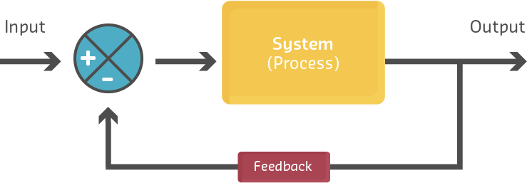
Understanding feedback control systems is essential for IoT device design. Most IoT applications require systems that can automatically maintain desired states without constant human intervention—this is the domain of closed-loop control.

TipKnowledge Check

Test your understanding of control system concepts.

NoteQuiz 1: Open-Loop vs Closed-Loop Control

Question 1: A basic sprinkler system waters the lawn for 15 minutes every morning at 6 AM, regardless of whether it rained overnight. A smart irrigation system uses soil moisture sensors to water only when moisture drops below 30%. Which classification is correct?

💡 Explanation: Open-loop systems operate based on predetermined inputs without measuring the output—the timer runs regardless of actual soil moisture. Closed-loop systems measure the output (soil moisture) and adjust the control action (watering) based on feedback. The key difference: open-loop cannot self-correct if conditions change (e.g., heavy rain); closed-loop automatically adapts. The timer sprinkler will waste water after rain; the smart system will skip watering because soil is already wet.

NoteQuiz 2: Feedback Loop Architecture

Question 2: In a closed-loop control system, the “error signal” is calculated as the difference between the setpoint and the measured value. If a heater setpoint is 25°C and the sensor reads 23°C, what is the error signal and what does it indicate?

💡 Explanation: Error = Setpoint - Measured = 25°C - 23°C = +2°C. A positive error means the actual value is below the desired setpoint, so the controller should increase the control action (more heating). A negative error would mean the actual value is above the setpoint (too hot). This sign convention is standard in control systems and determines the direction of the control response. The proportional term output would be: P = Kp × (+2°C) = positive value = increase heater power.

InlineKnowledgeCheck = FileAttachment("/assets/js/iotclass-inline-knowledgecheck.js").text().then(text => {
  eval(text);
  return window.InlineKnowledgeCheck;
})

214.5 Open-Loop vs Closed-Loop Systems

The fundamental distinction in control systems is whether they use feedback to adjust their behavior:

Figure 214.1: Open-loop control (top) operates without feedback, while closed-loop control (bottom) continuously measures output and adjusts to maintain desired setpoint

Detailed Comparison:

Feature	Open-Loop	Closed-Loop
Feedback	None—operates based on predetermined inputs	Continuous—measures output and adjusts
Accuracy	Low—cannot correct for disturbances	High—self-corrects to maintain setpoint
Complexity	Simple—fewer components, easier to design	More complex—requires sensors and control logic
Cost	Lower—no sensor feedback required	Higher—additional sensors and processing
Reliability	Susceptible to drift and external changes	Robust to disturbances and component variations
Speed	Can be fast (no feedback delays)	Slower (must wait for feedback measurements)
Energy	Less power (no continuous sensing)	More power (continuous sensing and adjustment)
IoT Example	Timer-based irrigation (waters for fixed duration)	Soil moisture-based irrigation (waters until target moisture reached)
Use Case	Predictable environments, low criticality	Variable environments, high accuracy needs

Real-World Examples:

Figure 214.2: Open-loop example (top): Microwave timer runs for fixed duration regardless of food temperature. Closed-loop example (bottom): Thermostat continuously measures room temperature and adjusts heater to maintain 22°C setpoint

Key Insight: Open-loop systems are predictable but inflexible—they cannot adapt to changing conditions. Closed-loop systems are adaptive but require more resources (sensors, processing, energy).

InlineKnowledgeCheck({
  id: "rtos-scheduling-algorithms",
  question: "A real-time IoT system runs on FreeRTOS with these tasks: **Emergency stop** (10ms period, 2ms execution, deadline=period), **Motor control** (20ms period, 5ms execution), **Sensor fusion** (50ms period, 8ms execution), **Data logging** (100ms period, 15ms execution). Which scheduling algorithm ensures all deadlines are met?",
  options: [
    "Round-robin (RR) - each task gets equal 25ms time slice, fair CPU sharing",
    "First-Come-First-Served (FCFS) - tasks execute in arrival order, simple implementation",
    "Rate-Monotonic Scheduling (RMS) - priority assigned by period (shorter period = higher priority)",
    "Earliest Deadline First (EDF) - dynamically prioritize task with nearest absolute deadline"
  ],
  correctIndex: 2,
  explanation: "**Rate-Monotonic Scheduling (RMS)** is correct for periodic real-time tasks: Assign priorities: Emergency stop (10ms period) = Highest, Motor control (20ms) = High, Sensor fusion (50ms) = Medium, Data logging (100ms) = Lowest. **Schedulability test**: CPU utilization = (2/10) + (5/20) + (8/50) + (15/100) = 0.2 + 0.25 + 0.16 + 0.15 = **76%**. RMS guarantee: If U ≤ n(2^(1/n) - 1), where n=4 tasks → 4(2^0.25 - 1) = 0.757 = **75.7%**. System is at **76%**, slightly above bound but often schedulable in practice (bound is sufficient but not necessary). **Why RR fails**: Equal time slices ignore urgency—emergency stop might miss 10ms deadline waiting for 25ms slice. **Why FCFS fails**: No preemption—if data logging (15ms) starts, emergency stop waits 15ms (misses 10ms deadline). **Why EDF is overkill**: Optimal for dynamic tasks but RMS is simpler for fixed periodic tasks (lower overhead, easier analysis). **Real FreeRTOS**: Uses priority-based preemptive scheduling—RMS maps directly to task priority levels. Configure: `xTaskCreate(EmergencyStop, priority=4)`, `xTaskCreate(MotorControl, priority=3)`, etc.",
  difficulty: "Advanced"
})

InlineKnowledgeCheck({
  id: "process-states-transitions",
  question: "An IoT task running on FreeRTOS is in **RUNNING** state executing sensor code. It calls `xSemaphoreTake()` to acquire a mutex that is currently held by another task. The mutex is not available. What state transition occurs, and what triggers the return to READY state?",
  options: [
    "RUNNING → READY → RUNNING (task remains in ready queue, scheduler tries again next tick)",
    "RUNNING → BLOCKED → READY → RUNNING (task blocks waiting for mutex; becomes READY when mutex released via xSemaphoreGive() by holder)",
    "RUNNING → SUSPENDED → RUNNING (task suspended until mutex available, no scheduler involvement)",
    "RUNNING → WAITING → READY → RUNNING (task enters waiting state for fixed timeout period)"
  ],
  correctIndex: 1,
  explanation: "Correct sequence: **RUNNING → BLOCKED → READY → RUNNING**. (1) **RUNNING → BLOCKED**: `xSemaphoreTake()` on unavailable mutex immediately blocks the task—removed from ready queue, placed in mutex's waiting list. Task does not consume CPU while blocked. (2) **BLOCKED → READY**: When mutex holder calls `xSemaphoreGive()`, RTOS moves blocked task to READY queue. Highest-priority ready task runs next (might be newly-unblocked task if priority > current task). (3) **READY → RUNNING**: Scheduler selects task from ready queue (if highest priority, runs immediately; otherwise waits turn). **Why READY-only fails**: Task would busy-wait checking mutex (wastes CPU, prevents lower-priority tasks from running). **Why SUSPENDED differs**: SUSPENDED is explicit pause via `vTaskSuspend()`—requires `vTaskResume()` call, not automatic on resource availability. **Why WAITING differs**: WAITING typically refers to timed delays (`vTaskDelay()`)—triggers on timer expiry, not external event. **Real FreeRTOS states**: RUNNING, READY, BLOCKED (waiting for resource/event), SUSPENDED (explicitly paused), DELETED (task removed).",
  difficulty: "Intermediate"
})

214.6 Real-World Example: Smart Factory Temperature Control

⭐⭐ Difficulty: Intermediate

Industry Context: A semiconductor manufacturing facility requires precise temperature control in clean rooms to maintain product quality. Even ±0.5°C variations can cause $50,000+ in defective wafer batches.

System Components:

Component	Specification	Cost	Function
Temperature Sensors	±0.1°C accuracy, PT1000 RTD	$85 each × 12	Measure zone temperatures
HVAC Actuators	Modulating dampers, 0-10V control	$450 each × 4	Regulate airflow
Edge Controller	Siemens S7-1200 PLC	$800	Execute PID control loops
Cloud Dashboard	Azure IoT Central	$200/month	Monitoring and analytics

Process Flow:

%%{init: {'theme': 'base', 'themeVariables': { 'primaryColor': '#2C3E50', 'primaryTextColor': '#fff', 'primaryBorderColor': '#16A085', 'lineColor': '#16A085', 'secondaryColor': '#E67E22', 'tertiaryColor': '#7F8C8D'}}}%%
flowchart TB
    subgraph Inputs[Clean Room Inputs]
        T1[Ambient Temperature]
        H1[Heat from Equipment]
        P1[Worker Body Heat]
        A1[HVAC Supply Air]
    end

    subgraph Process[Control Process - Edge PLC]
        S1[Read 12 Temp Sensors]
        C1[Calculate Zone Errors]
        P2[PID Controller<br/>Kp=3.5, Ki=0.2, Kd=1.2]
        O1[Output to Dampers]
    end

    subgraph Outputs[Controlled Outputs]
        R1[Room Temp: 22.0 C +/- 0.1 C]
        Q1[Product Quality: 99.7%]
        E1[Energy: 12 kWh/hr]
    end

    subgraph Feedback[Feedback Loop]
        M1[Measure Every 5 Seconds]
        Compare[Compare to 22.0 C Setpoint]
    end

    Inputs --> S1
    S1 --> C1
    C1 --> P2
    P2 --> O1
    O1 --> Outputs
    Outputs --> M1
    M1 --> Compare
    Compare --> C1

    style Inputs fill:#2C3E50,color:#fff
    style Process fill:#E67E22,color:#fff
    style Outputs fill:#16A085,color:#fff
    style Feedback fill:#7F8C8D,color:#fff

Figure 214.3: Clean Room PID Temperature Control System with Feedback Loop

Performance Metrics (Before vs After Closed-Loop Implementation):

Metric	Before (Manual Control)	After (Closed-Loop Control)	Improvement
Temperature Stability	±1.2°C variation	±0.08°C variation	93% reduction
Defect Rate	3.2% (640 defects/20k wafers)	0.3% (60 defects/20k wafers)	91% reduction
Annual Defect Cost	$960,000 ($1,500/defect)	$90,000	$870K saved
Energy Consumption	15.2 kWh/hr (over-cooling)	12.0 kWh/hr (optimized)	21% reduction
Response to Disturbance	12 minutes to stabilize	3 minutes to stabilize	75% faster
Operator Interventions	8 adjustments/shift	0.5 adjustments/shift	94% reduction

Key Insights:

1. Local Feedback is Critical: Edge PLC responds in <200ms. Cloud-only control would have 2-5 second latency—unacceptable for 5-second disturbances (door openings, equipment cycling).

2. System Decomposition: Clean separation of sensing (PT1000 RTDs), processing (PLC control algorithm), actuation (modulating dampers), and monitoring (Azure cloud) enabled modular upgrades without full replacement.

3. ROI Analysis: $12,220 total investment ($1,020 sensors + $1,800 actuators + $800 PLC + $600 cloud/3 months). Payback in 15 days from defect reduction alone ($870K annual savings ÷ 365 days = $2,384/day).

4. Feedback >> Open-Loop: Manual control (effectively open-loop with slow human feedback) caused ±1.2°C swings. Continuous sensor feedback reduced this to ±0.08°C—a 15× improvement.

214.7 Closed-Loop IoT System Diagram

Here’s a complete closed-loop control system architecture applied to an IoT smart thermostat:

Flowchart diagram

Figure 214.4: Complete closed-loop control system for IoT smart thermostat showing setpoint, error calculation, PID controller, actuator (HVAC), process (room heating), sensor (thermometer), and feedback loop

System Operation:

1. Setpoint: User sets desired temperature (22°C) via app or thermostat dial
2. Comparison: Summing junction compares setpoint to measured temperature from sensor
3. Error Calculation: If room is 18°C, error = 22°C - 18°C = +4°C (too cold)
4. Controller: Calculates control signal based on error magnitude
5. Actuator: HVAC system adjusts heating/cooling power based on control signal
6. Process: Room temperature changes due to HVAC output
7. Sensor: Thermometer measures actual room temperature
8. Feedback: Measured temperature fed back to summing junction → loop repeats

Continuous Cycle: This loop executes continuously (e.g., every 30 seconds) to automatically maintain 22°C despite disturbances (door openings, sunlight, occupancy changes).

%%{init: {'theme': 'base', 'themeVariables': {'primaryColor': '#2C3E50', 'primaryTextColor': '#fff', 'lineColor': '#16A085', 'secondaryColor': '#E67E22', 'tertiaryColor': '#7F8C8D'}}}%%
graph TB
    subgraph OpenLoop["OPEN-LOOP CONTROL"]
        OL_IN[User Input<br/>Run for 2 hours]
        OL_CTRL[Timer Controller]
        OL_ACT[Heater]
        OL_OUT[Room Temp<br/>Unknown result]

        OL_IN --> OL_CTRL
        OL_CTRL --> OL_ACT
        OL_ACT --> OL_OUT

        OL_PROB[Problem: No adaptation<br/>May overheat or underheat]
    end

    subgraph ClosedLoop["CLOSED-LOOP CONTROL"]
        CL_SP[Setpoint<br/>22 C target]
        CL_SUM((Compare))
        CL_CTRL[Controller]
        CL_ACT[HVAC System]
        CL_PROC[Room]
        CL_OUT[Actual Temp<br/>Measured result]
        CL_SENS[Sensor]

        CL_SP --> CL_SUM
        CL_SUM --> CL_CTRL
        CL_CTRL --> CL_ACT
        CL_ACT --> CL_PROC
        CL_PROC --> CL_OUT
        CL_OUT --> CL_SENS
        CL_SENS -->|Feedback| CL_SUM

        CL_BEN[Benefit: Self-adjusting<br/>Maintains 22 C automatically]
    end

    style OL_IN fill:#7F8C8D,color:#fff
    style OL_CTRL fill:#7F8C8D,color:#fff
    style OL_OUT fill:#E74C3C,color:#fff
    style OL_PROB fill:#E74C3C,color:#fff
    style CL_SP fill:#16A085,color:#fff
    style CL_SUM fill:#7F8C8D,color:#fff
    style CL_CTRL fill:#2C3E50,color:#fff
    style CL_OUT fill:#16A085,color:#fff
    style CL_SENS fill:#E67E22,color:#fff
    style CL_BEN fill:#16A085,color:#fff

Figure 214.5: Alternative view: Side-by-side comparison of open-loop (no feedback, unpredictable results) versus closed-loop control (continuous feedback, maintains setpoint). This comparison highlights why closed-loop systems are essential for reliable IoT automation.

CautionCommon Misconception: “More Feedback = Better Control”

Misconception: Adding more feedback loops and faster sampling rates always improves system performance.

Reality: Excessive feedback can cause instability, noise amplification, and wasted energy:

Problem 1: Too-Fast Feedback (Oversampling) - Example: Smart thermostat checking temperature every 100ms - Issue: HVAC systems have thermal inertia (heating takes 5-10 minutes) - Result: Controller sees no change → increases heating → overshoots → oscillates - Fix: Match sampling rate to system dynamics (check every 30-60 seconds)

Problem 2: Sensor Noise Amplification - Example: Soil moisture sensor with ±5% noise, sampled every second - Issue: Small noise fluctuations trigger irrigation on/off rapidly - Result: Valve wear, energy waste, inconsistent watering - Fix: Add moving average filter (average last 10 readings) before control decision

Problem 3: Cascaded Loops Instability - Example: Temperature controller → valve controller → motor controller - Issue: Each loop tries to “correct” the others’ actions - Result: System hunts/oscillates, never settles to stable state - Fix: Use hierarchical control with proper time-scale separation (outer loop 10× slower than inner)

Best Practices: - Match feedback rate to process dynamics: Slow systems (temperature) = slow feedback (10-60s), Fast systems (motor position) = fast feedback (1-10ms) - Filter sensor noise: Use moving average, median filter, or low-pass filter before control logic - Tune gains carefully: Start conservative (low gains), increase until system responds quickly without oscillation - Consider energy: Each sensor reading costs power—sample only as often as needed

Real IoT Example - Smart Irrigation: - Bad: Check soil moisture every 1 minute, water when <30% - Good: Check every 30 minutes (averaged over 5 readings), water when <25% for 3 consecutive checks

Rule of Thumb: Feedback interval should be 5-10× faster than the system’s settling time, but no faster (diminishing returns + wasted energy).

InlineKnowledgeCheck({
  id: "context-switching-overhead",
  question: "An ESP32 microcontroller (240 MHz, dual-core) runs an RTOS with 4 tasks: **Task A** (sensor reading, 100ms period), **Task B** (data processing, 50ms period), **Task C** (network transmission, 200ms period), **Task D** (display update, 500ms period). Each context switch takes 15 microseconds to save/restore registers and stack pointers. Over 1 second, approximately how much CPU time is spent on context switching?",
  options: [
    "0.15ms (0.015%) - negligible overhead, context switching is nearly free",
    "1.5ms (0.15%) - low overhead, well-optimized RTOS with minimal state saving",
    "15ms (1.5%) - moderate overhead, may impact real-time performance on time-critical tasks",
    "150ms (15%) - severe overhead, system spending more time switching than executing tasks"
  ],
  correctIndex: 1,
  explanation: "Calculate switches per second: Task A (1000ms÷100ms = 10 switches), Task B (1000÷50 = 20), Task C (1000÷200 = 5), Task D (1000÷500 = 2). Total = 37 switches/sec minimum. In practice, add RTOS tick interrupts (typically 100-1000 Hz)—assume 100 Hz = 100 switches/sec. Total ≈ **137 context switches/sec**. At 15µs each: 137 × 15µs = **2.05ms ≈ 0.2%** overhead. **Why this matters**: (1) **Real-time guarantees**: If Task A has 100ms deadline, losing 2ms to switching is acceptable. (2) **Battery life**: On battery-powered IoT, even 0.2% adds up over months. (3) **Scalability**: Doubling task count doubles overhead—10 tasks = 1% overhead. **Optimization strategies**: Use **event-driven design** instead of polling (reduces unnecessary wake-ups), increase tick period if sub-millisecond timing not needed (1000Hz tick → 100Hz tick saves 90% tick overhead), minimize task count (combine related functions). **Real RTOS data**: FreeRTOS context switch on Cortex-M4 (similar to ESP32) is 12-20µs depending on FPU usage.",
  difficulty: "Intermediate"
})

InlineKnowledgeCheck({
  id: "thread-vs-process-model",
  question: "An IoT gateway needs to handle multiple concurrent operations: MQTT message processing, database queries, HTTP API requests, and sensor data aggregation. The gateway runs Linux on a quad-core ARM processor with 2GB RAM. Which concurrency model is MOST appropriate?",
  options: [
    "Multi-process model - fork() separate processes for each connection, full memory isolation",
    "Multi-threaded model - pthread_create() threads sharing address space, lightweight context switching",
    "Event-driven single-threaded model - epoll/select with non-blocking I/O, zero context switching",
    "Hybrid model - worker thread pool for CPU-bound tasks, async I/O for network operations"
  ],
  correctIndex: 3,
  explanation: "**Hybrid model (Option D)** is optimal: Combine **async I/O event loop** (for MQTT, HTTP—I/O bound) with **worker thread pool** (for DB queries, aggregation—CPU bound). **Why hybrid wins**: (1) **I/O efficiency**: MQTT/HTTP spend 95% time waiting for network—async I/O handles 10,000+ connections on one thread. (2) **CPU utilization**: Database queries and aggregation are CPU-intensive—offload to worker threads to use all 4 cores. (3) **Memory efficiency**: Threads share memory (unlike processes)—important for 2GB constrained system. **Why pure processes fail**: Each fork() copies ~50MB memory × 1000 connections = 50GB (swapping/OOM). Context switch: 5-10× slower than threads. **Why pure threads struggle**: 1000 threads × 8MB stack = 8GB memory. Contention on shared resources. **Why pure event-loop fails**: Blocking DB query stalls entire event loop—all connections freeze. **Implementation**: Use **libuv** or **tokio** (Rust) for async I/O, maintain 4-8 worker threads (1-2× CPU cores). **Real example**: Node.js uses this model—event loop for I/O, libuv thread pool for crypto/filesystem.",
  difficulty: "Advanced"
})

TipCross-Hub Connections

Interactive Learning Tools: - Simulations Hub - Try control system simulations to see feedback loops in action - Videos Hub - Watch process control demonstrations showing real controllers, feedback loops, and system stability concepts in action - Quizzes Hub - Test your understanding of open-loop vs closed-loop systems and feedback mechanisms

Knowledge Resources: - Knowledge Gaps Hub - Common misconceptions about control systems and feedback loops - Knowledge Map - See how control types connect to sensors, actuators, and system architecture

NoteRelated Chapters

This Series: - Processes & Systems: Core Definitions - What are processes and systems - Processes & Systems: PID Control - PID controller theory and applications

Deep Dives: - Process Control and PID - Advanced feedback control systems - Processes Labs and Review - Hands-on implementations

Foundation: - IoT Reference Models - System architecture layers - Architectural Enablers - IoT technology stack

Sensing & Actuation: - Sensor Fundamentals - Input devices - Actuators - Output devices

214.8 Summary

This chapter covered the fundamentals of control types in IoT systems:

• Open-Loop vs Closed-Loop Control: Distinguishing between systems that operate without feedback (open-loop) and those that continuously measure and adjust based on output (closed-loop)
• Feedback Control Systems: Understanding how closed-loop systems use sensors to measure outputs, compare to desired setpoints, and adjust actuators to maintain target behavior
• Error Signal Calculation: Learning how error = setpoint - measured value determines control direction and magnitude
• System Stability: Recognizing that feedback must be matched to system dynamics to avoid oscillations and instability
• Noise and Filtering: Understanding that sensor noise requires filtering before use in control decisions
• Real-World Applications: Applying control concepts to smart factory temperature control, irrigation systems, and HVAC automation
• Design Trade-offs: Evaluating accuracy vs complexity, cost vs reliability, and speed vs energy consumption

214.9 What’s Next

The next chapter explores PID Control for IoT, diving deep into Proportional-Integral-Derivative (PID) control theory, the mathematical foundation for feedback systems. You’ll learn how to tune PID controllers for stability, analyze system response curves, and implement control algorithms for real IoT applications like temperature regulation and motor control.