%%{init: {'theme': 'base', 'themeVariables': { 'primaryColor': '#2C3E50', 'primaryTextColor': '#fff', 'primaryBorderColor': '#16A085', 'lineColor': '#16A085', 'secondaryColor': '#E67E22', 'tertiaryColor': '#ecf0f1', 'fontSize': '15px'}}}%%
graph TB
    Error["Error<br/>e(t)"] -->|Accumulate<br/>Over Time| Int["Integral<br/>∫e(t) dt"]
    Int -->|Multiply by Ki| Gain["Integral<br/>Gain<br/>Ki"]
    Gain -->|Output = Ki × ∫e dt| Output["Control<br/>Output<br/>u_i(t)"]

    Persist["Persistent<br/>Small Error<br/>e = 0.5°C"] -.->|"Accumulates:<br/>0.5+0.5+0.5..."| Growing["Growing<br/>Integral<br/>Output"]
    Growing -.->|"Increases Until<br/>Error = 0"| Zero["Zero<br/>Steady-State<br/>Error"]

    style Error fill:#E67E22,stroke:#16A085,stroke-width:2px,color:#fff
    style Int fill:#2C3E50,stroke:#16A085,stroke-width:2px,color:#fff
    style Gain fill:#2C3E50,stroke:#16A085,stroke-width:2px,color:#fff
    style Output fill:#16A085,stroke:#2C3E50,stroke-width:2px,color:#fff
    style Zero fill:#16A085,stroke:#2C3E50,stroke-width:3px,color:#fff
233 Integral and Derivative Control
233.1 Learning Objectives
By the end of this chapter, you will be able to:
- Explain how integral control eliminates steady-state error
- Identify and mitigate integral windup problems
- Describe how derivative control reduces overshoot and provides damping
- Compare P-only, PI, and PID control configurations
- Select the appropriate PID configuration for different applications
233.2 Integral Control (I)
The Integral term accumulates error over time and provides control action based on the total accumulated error. This eliminates steady-state error that P-only control cannot handle.
\[ u_i(t) = K_i \cdot \int_{0}^{t} e(\tau) \, d\tau \]
Integral Control Mechanism: Accumulates error over time. Even small persistent errors grow the integral, increasing control output until error reaches exactly zero. Eliminates steady-state offset that P-only cannot fix.
How Integral Control Works:
- Accumulates error over time: \(\int e(t) dt\)
- If error persists (even small error), integral grows
- Integral keeps increasing until error becomes zero
- Also called “automatic reset” - resets bias until error eliminated
Mathematical Intuition:
The integral accumulates (sums) all past errors:
Time | Error | Proportional | Integral Accumulated | Total Output
-----|-------|-------------|---------------------|-------------
0s   | +3C   | Kp×3 = 1.5  | 0                   | 1.5
1s   | +2C   | Kp×2 = 1.0  | Ki×(3+2) = 0.5      | 1.5
2s   | +1C   | Kp×1 = 0.5  | Ki×(3+2+1) = 0.6    | 1.1
3s   | +1C   | Kp×1 = 0.5  | Ki×(3+2+1+1) = 0.7  | 1.2
4s   | 0C    | Kp×0 = 0    | Ki×(3+2+1+1+0) = 0.7| 0.7
5s   | 0C    | Kp×0 = 0    | Ki×(3+2+1+1+0+0)=0.7| 0.7

Kp = 0.5, Ki = 0.1
Key Observations: - Even when P term drops to zero (error = 0), I term maintains output - This compensates for disturbances requiring sustained control action - Integral prevents steady-state error
Benefits of Adding Integral:
- Eliminates steady-state error: System reaches exact set point
- Compensates for disturbances: Overcomes constant external forces
- Automatic adjustment: No manual reset needed
Cautions with Integral:
- Integral Windup: Integral can accumulate excessively during large errors
- Slower Response: Can slow down initial response
- Overshoot: Can cause overshoot if Ki too large
- Requires Careful Tuning: Ki must be chosen carefully
233.3 Derivative Control (D)
The Derivative term provides control action based on the rate of change of error. It anticipates future error trends and provides damping to prevent overshoot.
\[ u_d(t) = K_d \cdot \frac{de(t)}{dt} \]
%%{init: {'theme': 'base', 'themeVariables': { 'primaryColor': '#2C3E50', 'primaryTextColor': '#fff', 'primaryBorderColor': '#16A085', 'lineColor': '#16A085', 'secondaryColor': '#E67E22', 'tertiaryColor': '#ecf0f1', 'fontSize': '15px'}}}%%
graph TB
    Error["Error<br/>e(t)"] -->|Calculate Rate<br/>of Change| Deriv["Derivative<br/>de(t)/dt"]
    Deriv -->|Multiply by Kd| Gain["Derivative<br/>Gain<br/>Kd"]
    Gain -->|Output = Kd × de/dt| Output["Control<br/>Output<br/>u_d(t)"]

    Fast["Error Decreasing<br/>Rapidly<br/>de/dt = -2°C/s"] -.->|Negative<br/>Derivative| Brake["Negative Output<br/>(Reduce Control)<br/>Prevents Overshoot"]
    Slow["Error Stable<br/>de/dt = 0"] -.->|Zero<br/>Derivative| None["No D<br/>Contribution"]

    style Error fill:#E67E22,stroke:#16A085,stroke-width:2px,color:#fff
    style Deriv fill:#2C3E50,stroke:#16A085,stroke-width:2px,color:#fff
    style Gain fill:#2C3E50,stroke:#16A085,stroke-width:2px,color:#fff
    style Output fill:#16A085,stroke:#2C3E50,stroke-width:2px,color:#fff
    style Brake fill:#16A085,stroke:#2C3E50,stroke-width:3px,color:#fff
Derivative Control Mechanism: Measures rate of error change. Rapid error decrease (approaching target fast) produces negative D output, reducing control action preemptively to prevent overshoot. Acts as predictive damping brake.
How Derivative Control Works:
- Measures how fast error is changing: \(\frac{de}{dt}\)
- If error decreasing rapidly, derivative is negative
- Negative derivative reduces control action (anticipates reaching target)
- Provides damping effect to prevent overshoot
- Acts as predictive brake
Derivative Calculation Example:
Time | Error | Error Change | P Output | I Output | D Output | Total
-----|-------|--------------|----------|----------|----------|------
0s   | +5C   | —            | 2.5      | 0        | 0        | 2.5
1s   | +4C   | -1C/s        | 2.0      | 0.45     | -0.3     | 2.15
2s   | +2C   | -2C/s        | 1.0      | 0.55     | -0.6     | 0.95
3s   | +0.5C | -1.5C/s      | 0.25     | 0.6      | -0.45    | 0.4
4s   | 0C    | -0.5C/s      | 0        | 0.6      | -0.15    | 0.45
5s   | 0C    | 0C/s         | 0        | 0.6      | 0        | 0.6

Kp = 0.5, Ki = 0.05, Kd = 0.3
Error Change = (Current Error - Previous Error) / Δt
Key Observations: - When error decreases rapidly (large negative de/dt), D term is negative - Negative D term reduces total output, slowing approach - As approach slows (de/dt approaches 0), D term reduces to zero - D acts as damping, preventing overshoot from P and I
Benefits of Adding Derivative:
- Reduces overshoot: Dampens aggressive P and I responses
- Improves stability: Prevents oscillations
- Faster settling: Reaches steady state more quickly
- Better response to changing conditions: Anticipates trends
Cautions with Derivative:
- Noise sensitivity: Amplifies high-frequency noise in sensor readings
- Difficult to tune: Kd selection is challenging
- Rarely used alone: Almost always combined with P and/or I
- May prevent reaching target: Excessive Kd can slow response too much
233.4 PID Control Summary
%%{init: {'theme': 'base', 'themeVariables': { 'primaryColor': '#2C3E50', 'primaryTextColor': '#fff', 'primaryBorderColor': '#16A085', 'lineColor': '#16A085', 'secondaryColor': '#E67E22', 'tertiaryColor': '#ecf0f1', 'fontSize': '15px'}}}%%
graph TB
    SP["Setpoint"] --> Comp["Error<br/>Calculation"]
    Meas["Measured<br/>Value"] --> Comp

    Comp -->|"e(t)"| P["P: Present<br/>Kp × e(t)<br/>Fast Response"]
    Comp -->|"∫e dt"| I["I: Past<br/>Ki × ∫e dt<br/>Eliminate Offset"]
    Comp -->|"de/dt"| D["D: Future<br/>Kd × de/dt<br/>Prevent Overshoot"]

    P --> Sum["Σ<br/>Combined<br/>Output"]
    I --> Sum
    D --> Sum

    Sum -->|"u(t) = P + I + D"| Plant["Process"]
    Plant --> Meas

    style Comp fill:#E67E22,stroke:#16A085,stroke-width:2px,color:#fff
    style P fill:#2C3E50,stroke:#16A085,stroke-width:2px,color:#fff
    style I fill:#2C3E50,stroke:#16A085,stroke-width:2px,color:#fff
    style D fill:#2C3E50,stroke:#16A085,stroke-width:2px,color:#fff
    style Sum fill:#16A085,stroke:#2C3E50,stroke-width:3px,color:#fff
    style Plant fill:#7F8C8D,stroke:#16A085,stroke-width:2px,color:#fff
Complete PID Controller Architecture: Error drives three parallel control actions. P term addresses present error (fast), I term corrects accumulated past error (accuracy), D term anticipates future trends (stability). Combined output creates optimal control signal.
Response Comparison:
%%{init: {'theme': 'base', 'themeVariables': { 'primaryColor': '#2C3E50', 'primaryTextColor': '#fff', 'primaryBorderColor': '#16A085', 'lineColor': '#16A085', 'secondaryColor': '#E67E22', 'tertiaryColor': '#ecf0f1', 'fontSize': '14px'}}}%%
graph LR
    subgraph POnly ["P-Only"]
        P1["Fast<br/>Response"] --> P2["Steady-State<br/>Error<br/>Remains"]
    end

    subgraph PI ["PI Control"]
        I1["Good<br/>Response"] --> I2["Zero<br/>Steady-State<br/>Error"]
        I2 --> I3["Possible<br/>Overshoot"]
    end

    subgraph PID ["PID Control"]
        D1["Fast<br/>Response"] --> D2["Zero<br/>Steady-State<br/>Error"]
        D2 --> D3["Minimal<br/>Overshoot<br/>Best Performance"]
    end

    style P2 fill:#E74C3C,stroke:#2C3E50,stroke-width:2px,color:#fff
    style I3 fill:#E67E22,stroke:#16A085,stroke-width:2px,color:#fff
    style D3 fill:#16A085,stroke:#2C3E50,stroke-width:3px,color:#fff
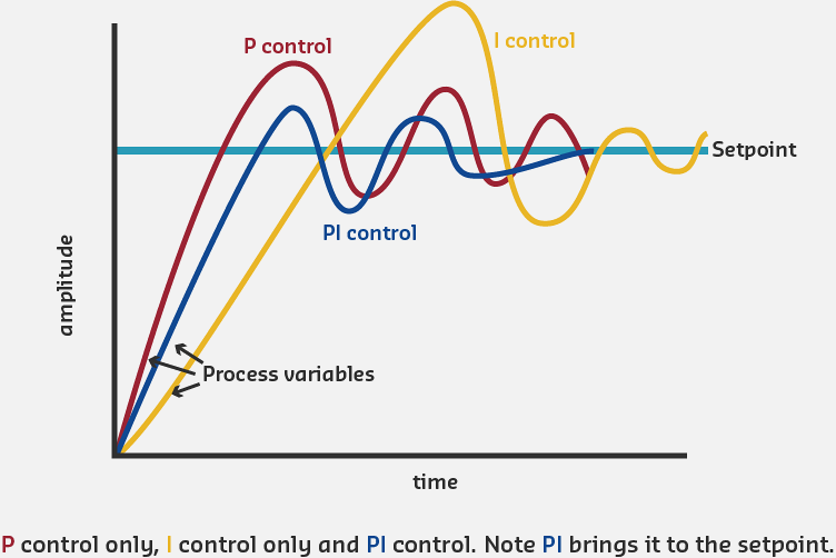
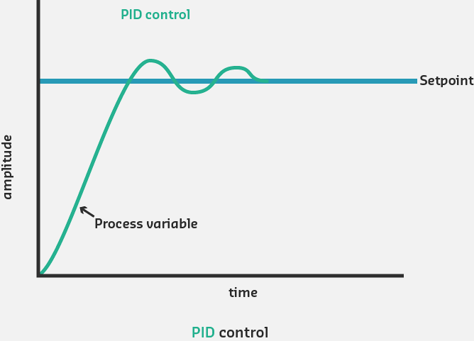
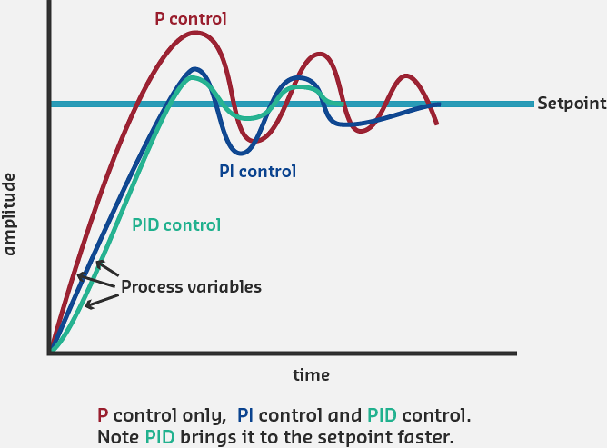
PID Configuration Performance Comparison: P-only provides fast response but leaves steady-state error. PI eliminates error but may overshoot. Full PID combines fast response, zero error, and minimal overshoot for optimal performance.
When to Use Each Configuration:
- P Only: Simple systems, fast response needed, some error acceptable
- PI: Most common, general-purpose control, steady-state accuracy required
- PID: High-performance applications, minimal overshoot critical
- PD: Rare, fast servos with no steady-state error concerns
233.5 Visual Reference Gallery
NoteVisual: Feedback System with Example

NoteVisual: Drone Flight Control System

NoteVisual: PID Derivative Action

233.6 Summary
This chapter covered the Integral and Derivative components of PID control:
Key Takeaways:
Integral Control (I): Accumulates error over time to eliminate steady-state error that P-only control cannot address
Integral Windup: A dangerous condition where the integral accumulates excessively during prolonged errors - requires anti-windup mechanisms
Derivative Control (D): Responds to the rate of error change, providing predictive braking to reduce overshoot
D Term Limitations: Sensitive to sensor noise and difficult to tune - often omitted in favor of PI control
Configuration Selection: PI is most common for general-purpose control; full PID only needed when minimal overshoot is critical
Tuning Philosophy: Conservative, balanced gains outperform aggressive tuning in real-world conditions
233.7 What’s Next?
In the next chapter, we’ll explore hands-on PID implementation with labs, Arduino/ESP32 code examples, and production-ready frameworks.