%% fig-alt: "Diagram showing IoT architecture components and their relationships with data flow and processing hierarchy."
%%{init: {'theme': 'base', 'themeVariables': { 'primaryColor': '#2C3E50', 'primaryTextColor': '#fff', 'primaryBorderColor': '#16A085', 'lineColor': '#16A085', 'secondaryColor': '#E67E22', 'tertiaryColor': '#7F8C8D'}}}%%

graph TB
    subgraph Surface["Ocean Surface"]
        Buoy1[Surface Buoy<br/>Anchor]
        Buoy2[Surface Buoy<br/>Anchor]
        Gateway[Gateway<br/>Satellite Uplink]
    end

    subgraph Underwater["Underwater Network - Acoustic Communication"]
        Sub1[Sensor Node 1]
        Sub2[Sensor Node 2]
        Sub3[Sensor Node 3]
        AUV[AUV Mobile<br/>Collector]
    end

    Sub1 & Sub2 & Sub3 -.->|Acoustic<br/>1500 m/s| AUV
    AUV -.->|Acoustic| Buoy1
    Buoy1 -->|Radio| Gateway
    Buoy2 -.->|Acoustic<br/>Localization| Sub2

    style Sub1 fill:#16A085,stroke:#2C3E50,color:#fff
    style Sub2 fill:#16A085,stroke:#2C3E50,color:#fff
    style Sub3 fill:#16A085,stroke:#2C3E50,color:#fff
    style AUV fill:#E67E22,stroke:#2C3E50,color:#fff
    style Buoy1 fill:#2C3E50,stroke:#16A085,color:#fff
    style Buoy2 fill:#2C3E50,stroke:#16A085,color:#fff
    style Gateway fill:#2C3E50,stroke:#16A085,color:#fff
400 Underwater Acoustic Sensor Networks (UWASNs)
TipFor Beginners: Talking Underwater Like Dolphins
Have you ever tried to use a walkie-talkie underwater? It doesn’t work! Radio waves can’t travel through water - they get absorbed almost immediately. So how do submarines communicate? The same way dolphins and whales do - with sound!
Underwater Sound Facts: - Sound travels about 1,500 meters per second in water (that’s faster than in air, but 200,000 times slower than radio!) - A message traveling 1 kilometer underwater takes almost 1 second to arrive - By the time your message arrives, a fast-moving fish might be 10 meters away from where you detected it!
| Term | Simple Explanation |
|---|---|
| UWASN | Underwater Acoustic Sensor Network - uses sound instead of radio |
| Acoustic Communication | Talking underwater using sound waves (like whales!) |
| AUV | Autonomous Underwater Vehicle - a robot submarine |
| Propagation Delay | The time it takes for a sound to travel from sender to receiver |
| Multipath | Sound bouncing off the surface and seafloor, causing echoes |
| Trilateration | Finding location using distances from multiple known points |
Why this matters: Underwater sensor networks monitor oil pipelines, track submarines, study marine life, and detect tsunamis. The slow speed of sound makes tracking underwater targets much harder than on land!
400.1 Learning Objectives
By the end of this chapter, you will be able to:
- Understand Acoustic Communication: Explain why radio doesn’t work underwater and how acoustic communication differs
- Analyze Propagation Delays: Calculate latency impact on tracking accuracy for underwater targets
- Model Oceanic Forces: Describe how currents, waves, and tides affect underwater node mobility
- Apply HASL Protocol: Explain High-Speed AUV-Based Silent Localization for energy-efficient positioning
- Design Opportunistic Localization: Plan iterative localization strategies with minimal infrastructure
- Compensate for Latency: Apply motion prediction techniques for stale position estimates
400.2 Prerequisites
Before diving into this chapter, you should be familiar with:
- Wireless Sensor Networks: Understanding of WSN architecture and communication basics
- WSN Tracking Fundamentals: Core tracking concepts including localization algorithms
- Wireless Multimedia Sensor Networks: Event-driven activation and energy optimization strategies
400.3 UWASN Characteristics
Underwater environments present unique challenges: no radio propagation, high latency, node mobility from ocean currents.
400.3.1 UWASN Architecture
Underwater Acoustic Sensor Network (UWASN) architecture showing acoustic communication (1500 m/s propagation creating high latency), surface buoy anchors for localization, mobile AUV for data collection, and gateway with satellite uplink. Challenges include multipath interference, Doppler shifts from currents, and limited bandwidth (1-10 kbps).
400.3.2 Key Challenges
| Challenge | Description | Impact |
|---|---|---|
| Acoustic propagation | Sound waves instead of radio | Low data rate (1-10 kbps) |
| High latency | Speed of sound: 1500 m/s | 0.67 ms per meter delay |
| Multipath | Reflections from surface/bottom | Signal distortion |
| Doppler effect | Node mobility causes frequency shifts | Difficult synchronization |
| Limited bandwidth | Acoustic channel: 1-100 kHz | Severe throughput limits |
| Energy constraints | Battery replacement very expensive | Must last years |
| Node mobility | Ocean currents move nodes | Dynamic topology |
400.3.3 Latency Impact on Tracking
Propagation speed comparison: - RF in air: 3 x 10^8 m/s (speed of light) - Acoustic in water: 1,500 m/s (200,000x slower!)
Latency calculations: - 1 km underwater: 1000m / 1500 m/s = 0.67 seconds delay - 5 km underwater: 3.37 seconds delay - Compare: 5 km RF in air = 0.000017 seconds (negligible)
Tracking challenge example: - Submarine moving at 10 m/s travels 33.7 meters during 3.37s delay - Position estimate is 33.7 meters stale by the time it reaches base station!
400.4 Oceanic Forces Mobility Model
Underwater nodes don’t move randomly - they’re affected by physical oceanographic forces:
%% fig-alt: "Diagram showing IoT architecture components and their relationships with data flow and processing hierarchy."
%%{init: {'theme': 'base', 'themeVariables': { 'primaryColor': '#2C3E50', 'primaryTextColor': '#fff', 'primaryBorderColor': '#16A085', 'lineColor': '#16A085', 'secondaryColor': '#E67E22', 'tertiaryColor': '#7F8C8D'}}}%%

graph TB
    subgraph Forces["Oceanographic Forces Acting on Underwater Nodes"]
        Current[Ocean Currents<br/>0.1-2 m/s horizontal]
        Wave[Wave Motion<br/>Sinusoidal vertical]
        Tide[Tidal Flows<br/>12-hour cycles]
        Thermal[Thermal Stratification<br/>Density layers]
    end

    subgraph Node["Underwater Sensor Node"]
        Buoy[Buoyancy Device]
        Sensor[Sensor Package]
        Anchor[Anchor Cable]
    end

    subgraph Effects["Movement Effects"]
        Horizontal[Horizontal Drift<br/>10-100m per day]
        Vertical[Vertical Oscillation<br/>plus/minus 1-5m per wave]
        Dynamic[Dynamic Topology<br/>Requires re-localization]
    end

    Current -->|Push| Node
    Wave -->|Lift| Node
    Tide -->|Pull| Node
    Thermal -->|Buoyancy| Node

    Node -->|Results in| Effects

    style Current fill:#16A085,stroke:#2C3E50,color:#fff
    style Wave fill:#16A085,stroke:#2C3E50,color:#fff
    style Tide fill:#16A085,stroke:#2C3E50,color:#fff
    style Thermal fill:#16A085,stroke:#2C3E50,color:#fff
    style Sensor fill:#E67E22,stroke:#2C3E50,color:#fff
    style Horizontal fill:#2C3E50,stroke:#16A085,color:#fff
    style Vertical fill:#2C3E50,stroke:#16A085,color:#fff
    style Dynamic fill:#2C3E50,stroke:#16A085,color:#fff
Oceanographic forces affecting underwater sensor node mobility: ocean currents (0.1-2 m/s horizontal drift), wave motion (sinusoidal vertical oscillation plus/minus 1-5m), tidal flows (12-hour cycles), and thermal stratification (density-driven buoyancy changes). Nodes can drift 10-100m per day, requiring frequent re-localization and creating dynamic network topology challenges.
Key mobility factors:
| Force | Effect | Magnitude |
|---|---|---|
| Ocean Currents | Horizontal drift | 0.1-2 m/s |
| Wave Motion | Vertical oscillation | plus/minus 1-5m per wave |
| Tidal Flows | Periodic displacement | 12-hour cycles |
| Thermal Stratification | Buoyancy changes | Density-driven vertical movement |
Result: Nodes can drift 10-100m per day, requiring frequent re-localization
400.5 3D Localization in UWASNs
GPS doesn’t work underwater. Localization requires acoustic ranging from surface anchors.
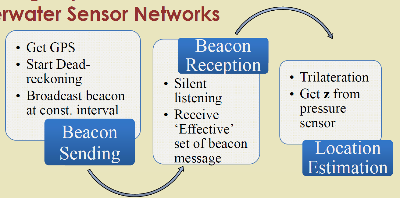
400.5.1 HASL Protocol
HASL (High-Speed AUV-Based Silent Localization):
%% fig-alt: "Diagram showing IoT architecture components and their relationships with data flow and processing hierarchy."
%%{init: {'theme': 'base', 'themeVariables': { 'primaryColor': '#2C3E50', 'primaryTextColor': '#fff', 'primaryBorderColor': '#16A085', 'lineColor': '#16A085', 'secondaryColor': '#E67E22', 'tertiaryColor': '#7F8C8D'}}}%%

sequenceDiagram
    participant AUV as AUV Mobile Anchor
    participant S1 as Sensor Node 1
    participant S2 as Sensor Node 2
    participant S3 as Sensor Node 3

    AUV->>AUV: Move to Position A<br/>(GPS-known)
    AUV->>S1: Broadcast Beacon<br/>(Position A, Time)
    AUV->>S2: Broadcast Beacon
    AUV->>S3: Broadcast Beacon

    Note over S1,S3: Nodes listen passively<br/>(Silent - No TX)

    S1->>S1: Measure ToA<br/>Calculate distance
    S2->>S2: Measure ToA<br/>Calculate distance
    S3->>S3: Measure ToA<br/>Calculate distance

    AUV->>AUV: Move to Position B
    AUV->>S1: Broadcast Beacon<br/>(Position B, Time)
    AUV->>S2: Broadcast Beacon
    AUV->>S3: Broadcast Beacon

    S1->>S1: Trilateration<br/>from A, B, C
    S2->>S2: Trilateration<br/>from A, B, C
    S3->>S3: Trilateration<br/>from A, B, C

    Note over S1,S3: Nodes localized<br/>without transmitting
HASL (High-Speed AUV-Based Silent Localization) protocol: AUV moves to multiple GPS-known positions broadcasting beacons, underwater sensor nodes passively listen and measure time-of-arrival to calculate distances, then perform trilateration. Silent operation (no sensor transmission) saves massive energy compared to traditional localization requiring sensor responses.
HASL Benefits: - Silent: Nodes listen passively (no transmission = energy savings) - Mobile anchor: AUV provides multiple reference positions - Scalable: Single AUV localizes many nodes in one pass
Energy savings calculation: - Traditional: 100 sensors x 100 beacon responses/hour = 10,000 transmissions/hour - HASL: 5 AUV broadcasts/hour = 5 transmissions/hour - 99.95% reduction in acoustic channel usage
400.5.2 Opportunistic Localization
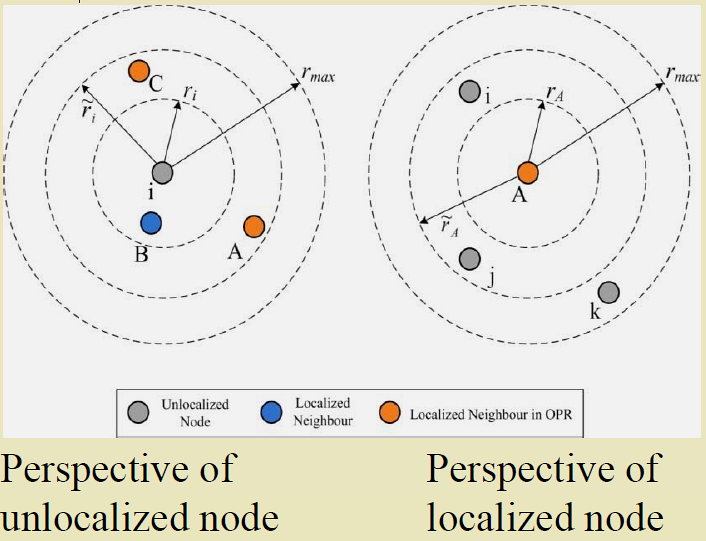
Strategy: Localized nodes assist in localizing nearby unlocalized nodes.
Iterative Localization: - Round 1: 3 surface anchors -> localize 5 nearby nodes - Round 2: 5 localized nodes -> localize 12 more - Round 3: 17 localized -> localize remaining - Result: Full network localization with only 3 surface anchors
How it works: 1. Initially localized nodes (anchored to surface buoys with GPS) broadcast their positions 2. Unlocalized nodes measure distances to multiple localized neighbors 3. Using trilateration, unlocalized nodes calculate their positions 4. Newly localized nodes can now assist others 5. Process iterates until all nodes are localized
400.6 Motion Prediction for Stale Estimates
Solution approaches for latency compensation:
- Kalman Filter Prediction: Use motion model to predict current position from stale measurements
- Extended Kalman Filter (EKF): Handles non-linear motion patterns underwater
- HASL Integration: Combine AUV-based localization with motion prediction
Example: Submarine Tracking
Measured position: (100m, 200m, 50m) at time T
Propagation delay: 3.37 seconds
Estimated velocity: (10 m/s, 0 m/s, 0 m/s)

Predicted current position:
  x = 100 + (10 * 3.37) = 133.7m
  y = 200 + (0 * 3.37) = 200m
  z = 50 + (0 * 3.37) = 50m

Predicted position: (133.7m, 200m, 50m)
400.7 Knowledge Check
TipQuestion: HASL Silent Localization
In underwater networks, HASL (High-Speed AUV-Based Silent Localization) uses mobile AUVs instead of fixed beacons. What makes the sensor nodes “silent” in this approach?
Options: - A) Sensors use optical signals instead of acoustic - B) Sensors only listen for AUV broadcasts; they do not transmit, saving massive energy - C) Sensors are physically quiet to avoid disturbing marine life - D) Sensors operate on low-frequency bands below audible range
NoteAnswer
Correct: B) Sensors only listen for AUV broadcasts; they do not transmit, saving massive energy
Traditional beacon localization (energy-expensive): 1. Fixed beacons broadcast positions periodically 2. Unknown nodes respond with measurements 3. Both sides transmit -> high energy consumption 4. Acoustic transmission is primary energy drain underwater
HASL silent localization: 1. AUV moves to GPS-known position (surfaces for GPS fix) 2. AUV broadcasts: “I am at position (x, y, z)” 3. Sensors LISTEN passively, measure time-of-arrival 4. Sensors calculate distance = sound_speed x time 5. Multiple AUV passes from different angles -> trilateration
Energy savings: - Traditional: 100 sensors x 100 beacon responses/hour = 10,000 transmissions/hour - HASL: 5 AUV broadcasts/hour = 5 transmissions/hour - 99.95% reduction in acoustic channel usage
Opportunistic extension: - Localized nodes assist unlocalized neighbors - Round 1: 3 surface anchors -> localize 5 nearby nodes - Round 2: 5 localized nodes -> localize 12 more - Round 3: Full network localization with minimal infrastructure
400.8 Visual Reference Gallery
NoteVisual: Underwater Sensor Networks

This visualization illustrates the underwater acoustic sensor network concepts covered in this chapter, showing acoustic propagation and AUV-based localization.
400.9 Summary
This chapter explored Underwater Acoustic Sensor Networks (UWASNs) and their unique challenges:
Acoustic Communication Fundamentals: - Sound travels at 1500 m/s underwater (200,000x slower than RF in air) - 1 km underwater link creates 0.67 second delay - Bandwidth limited to 1-10 kbps due to acoustic channel constraints
Major UWASN Challenges: - High Latency: Position estimates become stale during multi-second propagation delays - Multipath: Reflections from surface and seafloor distort signals - Node Mobility: Ocean currents drift nodes 10-100m per day - Energy Constraints: Battery replacement extremely expensive underwater
Localization Solutions: - HASL Protocol: AUV-based silent localization achieves 99.95% energy savings - Opportunistic Localization: Iterative positioning with minimal surface infrastructure - Motion Prediction: Kalman filtering compensates for stale position estimates
Oceanic Forces: - Currents: 0.1-2 m/s horizontal drift - Waves: Sinusoidal vertical oscillation - Tides: 12-hour periodic displacement - Thermal stratification: Density-driven buoyancy changes
Key Insights: - GPS doesn’t work underwater - must use acoustic ranging - Silent localization (receive-only sensors) dramatically reduces energy consumption - Motion prediction is essential for accurate tracking with multi-second delays
400.10 What’s Next
Continue to Nanonetworks to explore sensing and communication at molecular scales, enabling biomedical applications like targeted drug delivery and in-body health monitoring.