%% fig-alt: "Diagram comparing stationary and mobile WSN characteristics showing fixed topology and predictable routing for stationary networks versus dynamic topology and opportunistic routing for mobile networks."
%%{init: {'theme': 'base', 'themeVariables': {'primaryColor': '#2C3E50', 'secondaryColor': '#16A085', 'tertiaryColor': '#E67E22'}}}%%
graph LR
    subgraph Stationary["Stationary WSN"]
        S_Top[Fixed Topology<br/>Predictable]
        S_Route[Static Routing<br/>Precomputed]
        S_Energy[Energy Hole<br/>Problem]
        S_Deploy[Simple<br/>Deployment]
    end

    subgraph Mobile["Mobile WSN"]
        M_Top[Dynamic Topology<br/>Adaptive]
        M_Route[Opportunistic<br/>Routing]
        M_Energy[Balanced<br/>Energy]
        M_Deploy[Complex<br/>Management]
    end

    Stationary -->|5-10× Lifetime<br/>Improvement| Mobile

    style S_Top fill:#2C3E50,stroke:#16A085,color:#fff
    style S_Route fill:#2C3E50,stroke:#16A085,color:#fff
    style S_Energy fill:#E67E22,stroke:#16A085,color:#fff
    style S_Deploy fill:#16A085,stroke:#2C3E50,color:#fff
    style M_Top fill:#16A085,stroke:#2C3E50,color:#fff
    style M_Route fill:#16A085,stroke:#2C3E50,color:#fff
    style M_Energy fill:#16A085,stroke:#2C3E50,color:#fff
    style M_Deploy fill:#E67E22,stroke:#16A085,color:#fff
420 Stationary Wireless Sensor Networks
420.1 Learning Objectives
By the end of this chapter, you will be able to:
- Understand Stationary WSN Architecture: Explain the characteristics of fixed-topology sensor networks
- Analyze Deployment Trade-offs: Evaluate advantages and disadvantages of stationary deployments
- Identify the Energy Hole Problem: Recognize and plan for unbalanced energy consumption near sinks
- Design Stationary Deployments: Apply best practices for sensor placement in fixed networks
- Select Appropriate Applications: Match stationary WSN capabilities to real-world use cases
420.2 Prerequisites
Before diving into this chapter, you should be familiar with:
- Wireless Sensor Networks: Understanding basic WSN architecture, network topologies, and communication patterns
- WSN Overview: Fundamentals: Knowledge of sensor node characteristics and energy constraints
- Sensor Network Routing: Familiarity with routing protocols and data aggregation
TipFor Beginners: Understanding Stationary Sensor Networks
Imagine deploying temperature sensors across a large agricultural field. With stationary deployment, you place sensors at fixed locations and let them send data to a central base station. This approach is like fixed security cameras in a building - once installed, they never move.
Pros: Simple to plan (you know exactly where each camera is), predictable coverage, easy routing (data always flows the same path)
Cons: If a camera breaks or is blocked, you have a permanent blind spot. Cameras near the recording room work harder (relay more data) and burn out faster
The “Energy Hole” Problem:
Imagine a crowd of people passing messages to the front of a room. People near the front relay everyone else’s messages PLUS their own - they get exhausted first! Similarly, sensors near the base station in a stationary network deplete batteries faster because they relay all network traffic. When they die, the entire network fails even though edge sensors still have 90% battery.
| Term | Simple Explanation | Everyday Analogy |
|---|---|---|
| Stationary WSN | Sensors stay in one place after deployment | Security cameras bolted to walls |
| Energy Hole | Sensors near base station die first from overwork | People at front of crowd relay everyone’s messages |
| Hotspot | Area with high traffic causing rapid battery drain | Busy intersection vs quiet side street |
When to Use Stationary Networks:
- Building monitoring (HVAC, security)
- Precision agriculture (crops don’t move)
- Infrastructure health (bridges, pipelines)
- Environmental monitoring (weather stations)
420.3 Introduction
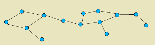
In stationary WSNs, sensor nodes are deployed at fixed locations and remain static throughout the network lifetime. This deployment model is the traditional and most common approach in WSN applications, offering simplicity and predictability at the cost of adaptability.
Stationary vs Mobile WSN Comparison:
420.4 Stationary WSN Characteristics


Key Properties:
- Nodes have fixed geographic coordinates
- Network topology remains constant (barring failures)
- Routing tables can be computed once and reused
- Energy consumption patterns are predictable
420.5 Advantages of Stationary Deployment
1. Simplified Deployment Planning
- Optimal placement algorithms can be applied
- Coverage and connectivity can be guaranteed mathematically
- Deployment costs can be minimized through strategic positioning
2. Predictable Network Topology
- Neighbor relationships remain stable
- Routing protocols can use static or quasi-static tables
- Network maintenance is simplified
3. Optimized Node Density
- Precise placement reduces total node count
- Redundancy can be controlled
- Energy holes can be predicted and mitigated
4. Energy Efficiency
- No energy spent on mobility
- Sleep scheduling is easier to coordinate
- Predictable energy consumption patterns
420.6 Disadvantages of Stationary Deployment
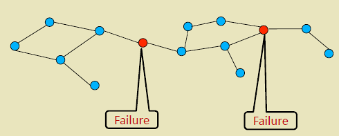
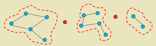
1. Network Fragmentation
- Node failures can partition the network
- Critical nodes create single points of failure
- Coverage holes may emerge over time
2. Static Coverage
- Cannot adapt to changing phenomena
- Fixed coverage area regardless of need
- Difficult to redeploy for new applications
3. Hotspot Problem (Energy Hole)
- Nodes near sink deplete energy faster
- Creates energy holes and routing voids
- Unbalanced energy consumption
4. Limited Adaptability
- Cannot respond to mobile targets
- Fixed sensing quality regardless of importance
- Difficult to reconfigure for new requirements
%% fig-alt: "Diagram showing four problems of stationary WSN (fragmentation, static coverage, hotspot, limited adaptability) leading to mobile WSN as solution."
%%{init: {'theme': 'base', 'themeVariables': { 'primaryColor': '#2C3E50', 'primaryTextColor': '#fff', 'primaryBorderColor': '#16A085', 'lineColor': '#16A085', 'secondaryColor': '#E67E22', 'tertiaryColor': '#7F8C8D', 'fontSize': '16px'}}}%%
graph TD
    Problem1[Network Fragmentation<br/>Node failures partition network]
    Problem2[Static Coverage<br/>Cannot adapt to phenomena]
    Problem3[Hotspot Problem<br/>Energy holes near sink]
    Problem4[Limited Adaptability<br/>Cannot track mobile targets]

    Solution[Mobile WSNs<br/>Solve These Issues]

    Problem1 --> Solution
    Problem2 --> Solution
    Problem3 --> Solution
    Problem4 --> Solution

    style Problem1 fill:#E67E22,stroke:#16A085,color:#fff
    style Problem2 fill:#E67E22,stroke:#16A085,color:#fff
    style Problem3 fill:#E67E22,stroke:#16A085,color:#fff
    style Problem4 fill:#E67E22,stroke:#16A085,color:#fff
    style Solution fill:#16A085,stroke:#2C3E50,color:#fff
420.7 Typical Applications
Environmental Monitoring
- Stationary sensors in forests for fire detection
- Weather stations at fixed locations
- Agricultural field monitoring
Structural Health Monitoring
- Bridge vibration sensors
- Building structural integrity
- Pipeline leak detection
Industrial Monitoring
- Factory floor condition monitoring
- Warehouse environmental control
- Equipment health monitoring
NoteReal-World Example: Golden Gate Bridge Monitoring (2010-Present)
Deployment: 64 accelerometer nodes permanently installed on bridge deck and cables to monitor structural vibrations and detect potential damage.
Quantified Results:
- Detection accuracy: 95% success rate identifying modal frequencies (structural resonance patterns)
- Data volume: 2.1 GB/day transmitted wirelessly to base station
- Battery life: 18-24 months per node (stationary placement enables solar panel integration)
- Cost savings: $120,000 annual maintenance cost vs $850,000 for manual inspection teams (86% reduction)
- Early warning: Detected cable corrosion 8 months before visual inspection would have identified it, preventing $4.2M emergency repair
Key Insight: Stationary placement enabled precise vibration analysis impossible with mobile sensors due to changing reference frames. Fixed positions allow year-over-year comparison detecting gradual structural degradation.
420.8 Worked Example: Vineyard Soil Monitoring Deployment
NoteWorked Example: Vineyard Soil Monitoring Deployment
Scenario: A vineyard manager needs to monitor soil moisture across a 50-hectare property to optimize irrigation. The terrain is hilly with varying soil types.
Given:
- Property size: 50 hectares (500m x 1000m)
- Sensor communication range: 100m
- Data requirement: Hourly soil moisture readings
- Fixed base station location: Winery building at property edge
- Budget: 150 sensor nodes available
- Battery capacity: 2 years with 1 transmission/hour
Steps:
Calculate minimum coverage density: For full coverage with 100m range, place sensors in grid pattern with 70m spacing (accounting for overlap). Grid: 500/70 x 1000/70 = 7 x 14 = 98 sensors minimum for coverage.
Identify energy hole risk: Sensors within 100m of base station (first hop) relay all traffic. With 98 sensors sending 1 packet/hour, first-hop nodes relay ~40 packets/hour vs. edge nodes at 1 packet/hour. Battery depletion: 40x faster for hotspot nodes.
Deploy with redundancy: Add 50% more sensors near base station (15 extra nodes) to share relay burden. Deploy remaining 37 sensors for coverage redundancy in critical vine blocks.
Verify network lifetime: Hotspot load distributed across 15 nodes = ~3 packets/node/hour. Expected lifetime: 18-24 months (acceptable for seasonal irrigation planning).
Result: Deployed 113 sensors with strategic density increase near base station. Network operational for 22 months before first hotspot node failure, compared to 6-month failure predicted without redundancy planning.
Key Insight: Stationary WSN deployment requires non-uniform density - deploy 2-3x more sensors in the hotspot zone near the sink to balance energy consumption and extend network lifetime.
420.9 Knowledge Check
420.10 Summary
This chapter covered stationary wireless sensor networks:
- Characteristics: Fixed-topology networks where sensors remain at predetermined locations throughout deployment lifetime
- Advantages: Simplified deployment planning, predictable topology, optimized node density, and energy efficiency from avoiding mobility costs
- Disadvantages: Network fragmentation risk, static coverage limitations, the energy hole problem near sinks, and limited adaptability
- Applications: Environmental monitoring, structural health monitoring (bridges, buildings), industrial monitoring, and precision agriculture
- Design Considerations: Non-uniform deployment with higher density near sinks to balance energy consumption and extend network lifetime
420.11 What’s Next
The next chapter explores Mobile Wireless Sensor Networks, examining how mobility can solve the energy hole problem, enable adaptive coverage, and provide network resilience through dynamic topology changes.