%% fig-alt: "Diagram comparing stationary WSN with fixed sensors and base station versus mobile WSN with moving sensors and mobile sink visiting different network regions."
%%{init: {'theme': 'base', 'themeVariables': { 'primaryColor': '#2C3E50', 'primaryTextColor': '#fff', 'primaryBorderColor': '#16A085', 'lineColor': '#16A085', 'secondaryColor': '#E67E22', 'tertiaryColor': '#7F8C8D', 'fontSize': '16px'}}}%%
graph LR
    subgraph "Stationary WSN"
        S1[Fixed<br/>Sensor] --- S2[Fixed<br/>Sensor]
        S2 --- S3[Fixed<br/>Sensor]
        S3 --> BS1[Base<br/>Station]
    end

    subgraph "Mobile WSN"
        M1[Sensor] -.Move.-> M2[Sensor]
        M2 -.Move.-> M3[Sensor]
        M_Sink[Mobile<br/>Sink] -.Visits.-> M1
        M_Sink -.Visits.-> M3
    end

    style S1 fill:#2C3E50,stroke:#16A085,color:#fff
    style S2 fill:#2C3E50,stroke:#16A085,color:#fff
    style S3 fill:#2C3E50,stroke:#16A085,color:#fff
    style BS1 fill:#E67E22,stroke:#16A085,color:#fff
    style M1 fill:#16A085,stroke:#2C3E50,color:#fff
    style M2 fill:#16A085,stroke:#2C3E50,color:#fff
    style M3 fill:#16A085,stroke:#2C3E50,color:#fff
    style M_Sink fill:#E67E22,stroke:#16A085,color:#fff
421 Mobile Wireless Sensor Networks (MWSNs)
421.1 Learning Objectives
By the end of this chapter, you will be able to:
- Understand MWSN Architecture: Explain how mobile sensor networks differ from stationary deployments
- Analyze Mobility Benefits: Evaluate how mobility solves the energy hole problem and enables adaptive coverage
- Apply Self-CHOP Properties: Design networks that self-configure, self-heal, self-optimize, and self-protect
- Evaluate Trade-offs: Balance mobility costs against benefits for specific applications
- Avoid Common Pitfalls: Recognize when mobility helps versus hurts network performance
421.2 Prerequisites
Before diving into this chapter, you should be familiar with:
- Stationary WSN Fundamentals: Understanding the energy hole problem and limitations of fixed deployments
- Wireless Sensor Networks: Basic WSN architecture and communication patterns
- Multi-Hop Ad Hoc: Fundamentals: Dynamic topologies and self-organizing networks
TipFor Beginners: Understanding Mobile Sensor Networks
Mobile Networks - Like Delivery Trucks:
Mobile sensor networks are like delivery trucks collecting packages:
- Mobile Sensors: Sensors themselves move (animal collars, vehicle-mounted sensors)
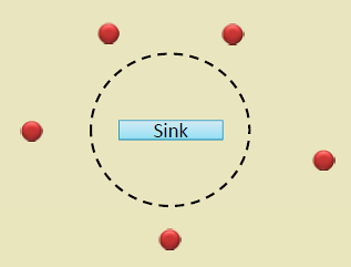
- Mobile Sinks: The “base station” moves around to collect data (bus driving past stationary sensors)
- Data MULEs: Special devices that ferry data (drone flying over sensors periodically)
Real-World Example: ZebraNet project attached GPS collars to zebras. Zebras move around all day storing location data. When two zebras meet, they exchange data. Eventually, a zebra comes near a base station at a watering hole and uploads all collected data. No fixed infrastructure needed!
| Term | Simple Explanation | Everyday Analogy |
|---|---|---|
| Mobile WSN | Sensors or collectors move around | Delivery truck picking up packages |
| Mobile Sink | Moving base station that visits sensors | Mail carrier walking route to collect mail |
| Data MULE | Device that physically carries data between points | USB drive carried between computers |
| Self-CHOP | Network self-configures, heals, optimizes, protects | Ant colony organizing without a central boss |
Why Mobility Helps:
Mobile sensor networks extend battery life by 5-10x compared to stationary networks by balancing the workload. However, they’re more complex to program and manage. Understanding the trade-offs helps you choose the right approach for your IoT application!
421.3 Introduction
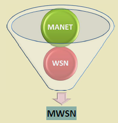
Mobile Wireless Sensor Networks (MWSNs) represent a paradigm shift where mobility is leveraged as a feature rather than a constraint. MWSNs inherit characteristics from Mobile Ad Hoc Networks (MANETs) while maintaining the sensing-centric nature of WSNs.
Basic Architecture Comparison:
NoteAlternative View: Stationary vs Mobile Selection Decision Tree
This variant shows when to choose stationary versus mobile WSN based on application requirements, helping architects make deployment decisions.
%% fig-alt: "Decision flowchart for WSN type selection: Start with target type. If monitoring fixed infrastructure like buildings, bridges, or pipelines, use stationary WSN. If tracking mobile targets like wildlife, vehicles, or people, use mobile WSN. For stationary, check if energy hole is acceptable. If yes, deploy simple stationary network. If no, consider mobile sink for energy balancing. For mobile, check if controlled mobility is possible. If yes like with drones or robots, use planned trajectory mobile WSN. If no like with animals or vehicles, use opportunistic mobile WSN with delay tolerance."
%%{init: {'theme': 'base', 'themeVariables': { 'primaryColor': '#2C3E50', 'primaryTextColor': '#fff', 'primaryBorderColor': '#16A085', 'lineColor': '#16A085', 'secondaryColor': '#E67E22', 'tertiaryColor': '#7F8C8D', 'fontSize': '14px'}}}%%
flowchart TD
    Start["WSN Application<br/>Requirements"] --> Target{Target<br/>Type?}

    Target -->|"Fixed Infrastructure<br/>(Buildings, Bridges)"| Stat1["STATIONARY WSN<br/>Predictable coverage"]
    Target -->|"Mobile Targets<br/>(Wildlife, Vehicles)"| Mobile1["MOBILE WSN<br/>Adaptive tracking"]

    Stat1 --> EnergyHole{Energy Hole<br/>Acceptable?}
    EnergyHole -->|"Yes<br/>(Short deployment)"| Simple["Simple Stationary<br/>Fixed sink"]
    EnergyHole -->|"No<br/>(Long lifetime)"| MobileSink["Stationary Sensors +<br/>Mobile Sink"]

    Mobile1 --> Control{Controlled<br/>Mobility?}
    Control -->|"Yes<br/>(Drones, Robots)"| Planned["Planned Trajectory<br/>Mobile WSN"]
    Control -->|"No<br/>(Animals, Vehicles)"| Opp["Opportunistic<br/>Mobile WSN"]

    style Start fill:#2C3E50,stroke:#16A085,color:#fff
    style Stat1 fill:#16A085,stroke:#2C3E50,color:#fff
    style Mobile1 fill:#E67E22,stroke:#2C3E50,color:#fff
    style Simple fill:#16A085,stroke:#2C3E50,color:#fff
    style MobileSink fill:#16A085,stroke:#2C3E50,color:#fff
    style Planned fill:#E67E22,stroke:#2C3E50,color:#fff
    style Opp fill:#E67E22,stroke:#2C3E50,color:#fff
Key Insight: The choice between stationary and mobile WSN is primarily driven by whether the monitoring target moves. For fixed targets, stationary WSN is simpler unless network lifetime is critical (then add mobile sink). For mobile targets, mobile WSN is required, with the type depending on whether you control the mobility.
421.4 Relationship with MANETs
MWSNs can be viewed as a specialized form of MANET with sensing capabilities:
Self-CHOP Properties (from MANET):
- Self-Configure: Nodes autonomously form network without infrastructure
- Self-Heal: Network recovers from node failures and topology changes
- Self-Optimize: Adapts routing and protocols to current conditions
- Self-Protect: Implements security mechanisms against attacks
WSN-Specific Properties:
- Large-scale dense deployment
- Energy-constrained operation
- Collaborative sensing and data aggregation
- Sink-oriented data flow
%% fig-alt: "Diagram showing MWSN as intersection of MANET (Self-CHOP properties) and WSN (dense deployment, energy constraints, data aggregation)."
%%{init: {'theme': 'base', 'themeVariables': { 'primaryColor': '#2C3E50', 'primaryTextColor': '#fff', 'primaryBorderColor': '#16A085', 'lineColor': '#16A085', 'secondaryColor': '#E67E22', 'tertiaryColor': '#7F8C8D', 'fontSize': '16px'}}}%%
graph TD
    MANET[Mobile Ad Hoc Network<br/>MANET] --> MWSN[Mobile WSN<br/>MWSN]
    WSN[Wireless Sensor Network<br/>WSN] --> MWSN

    MANET_Props[Self-CHOP Properties<br/>Configure, Heal, Optimize, Protect]
    WSN_Props[WSN Properties<br/>Dense deployment, Energy-constrained<br/>Data aggregation, Sink-oriented]

    MANET_Props --> MANET
    WSN_Props --> WSN

    style MANET fill:#E67E22,stroke:#16A085,color:#fff
    style WSN fill:#2C3E50,stroke:#16A085,color:#fff
    style MWSN fill:#16A085,stroke:#2C3E50,color:#fff
    style MANET_Props fill:#7F8C8D,stroke:#16A085,color:#fff
    style WSN_Props fill:#7F8C8D,stroke:#16A085,color:#fff
421.5 Advantages of Mobility


1. Adaptive Coverage
- Nodes move to areas requiring higher sensing density
- Dynamic coverage based on phenomenon importance
- Self-healing through mobility
2. Network Resilience
- Topology changes naturally overcome failures
- Alternative paths emerge through movement
- Reduced impact of single node failures
3. Target Tracking
- Mobile sensors follow moving targets
- Maintain optimal sensing distance
- Coordinate movement for multi-target tracking
4. Energy Balancing
- Mobile sink distributes hotspot load
- Nodes share burden through rotation
- Extended network lifetime
5. Enhanced Connectivity
- Mobile nodes act as data ferries
- Bridge disconnected partitions
- Opportunistic communication
421.6 Worked Example: Mobile Sink Path Optimization
NoteWorked Example: Mobile Sink Path Optimization for Precision Agriculture
Scenario: A vineyard wants to extend network lifetime beyond 2 years by adding a mobile sink mounted on an autonomous tractor that already traverses the property daily for spraying operations.
Given:
- 113 stationary soil sensors from previous deployment
- Tractor path: Covers all vine rows over 8-hour daily operation
- Tractor speed: 5 km/h average
- Communication range: 100m (sensors to mobile sink)
- Original network lifetime with fixed sink: 22 months
- Target: 5+ year network lifetime
Steps:
Analyze original traffic pattern: Each sensor generates 24 packets/day. With fixed sink, hotspot sensors relay 960 packets/day (40 sensors x 24 packets). Transmission energy: 0.5 mJ/packet.
Calculate mobile sink benefit: When tractor passes within 100m, sensors transmit directly (1 hop) vs. average 4 hops to fixed sink. Energy savings: 4x per packet for distant sensors, relay burden eliminated for all sensors.
Verify tractor coverage: 8-hour operation at 5 km/h = 40 km path length. With 100m communication range, tractor “sweeps” 40 km x 200m = 8 km² = 80 hectares. Full coverage achieved since vineyard is 50 hectares.
Estimate new lifetime: Without relay burden, all sensors transmit only their own data (24 packets/day). Energy consumption uniform across network at 12 mJ/day vs. original hotspot at 480 mJ/day. Lifetime extension: 40x for former hotspot nodes.
Result: Network lifetime extended from 22 months to 7+ years. Zero additional energy cost since tractor already traverses property. Sensors report when tractor passes nearby (1-3 times daily), providing sufficient temporal resolution for irrigation decisions.
Key Insight: Mobile sinks are most effective when leveraging existing mobility (tractors, delivery vehicles, buses) rather than deploying dedicated mobile platforms. The “free” mobility eliminates the energy hole problem without adding operational complexity.
421.7 Common Misconceptions and Pitfalls
WarningCommon Misconception: “Mobile WSNs Always Extend Network Lifetime”
The Misconception: Many students assume that adding mobility to a sensor network automatically extends its lifetime because mobile sinks balance energy consumption. This oversimplification ignores the energy cost of mobility itself.
The Reality - Energy Trade-offs:
While mobile sinks can extend network lifetime by 5-10x, this only occurs when mobility energy cost < energy savings from reduced multi-hop communication.
When Mobile Sinks Help:
- Mobility is “free” (bus, tractor, animal already moving)
- High multi-hop relay burden in stationary deployment
- Low-duty-cycle mobility (infrequent visits sufficient)
- Energy-rich mobile platform (vehicle battery)
When Mobile Sinks Hurt:
- Mobility requires dedicated energy-constrained robot
- Network density low (few relay hops even with stationary sink)
- Continuous mobility required (high energy cost)
- Mobile platform has smaller battery than sensors
Design Rule: Only deploy mobile sinks when (Multi-hop energy savings) > (Mobility energy cost + System complexity cost). Otherwise, accept the stationary energy hole and just replace hotspot node batteries periodically!
CautionPitfall: Forming Network Topology Before Nodes Settle
The Mistake: Immediately after deployment, nodes run neighbor discovery and form routing trees. Hours later, environmental conditions change (temperature, humidity, obstacles) and 40% of established routes have poor link quality. The network wastes energy on retransmissions.
Why It Happens: Radio propagation varies significantly with conditions. Initial measurements during dry daytime deployment don’t reflect nighttime dew (6-12 dB attenuation), rain (up to 20 dB loss at 2.4 GHz), or thermal effects on antenna impedance.
The Fix: Implement a settling period and continuous link quality monitoring:
- Settling period: Wait 24-72 hours after deployment before finalizing routing topology
- Link quality sampling: Measure RSSI and packet reception rate (PRR) across multiple time windows
- Formation threshold: Only establish routes with PRR > 90% across all sampled conditions
- Margin requirement: Design for 10-15 dB link margin above receiver sensitivity
CautionPitfall: Aggregating Incompatible Data Types at Cluster Heads
The Mistake: A cluster head receives temperature readings from 20 nodes and transmits the average (21.3 C) to save energy. But one node detected a fire (85 C), and the critical alarm is lost - averaged away with normal readings.
Why It Happens: Developers apply generic aggregation (MIN/MAX/AVG/SUM) without considering data semantics. Averaging works for environmental monitoring but destroys anomaly information.
The Fix: Implement semantics-aware aggregation with anomaly preservation:
- Statistical aggregation: Send both mean AND variance - high variance signals potential anomalies
- Threshold preservation: Before averaging, check if ANY reading exceeds alarm threshold
- Spatial coherence check: Compare readings within cluster - skip aggregation if CV > 0.3
- Data type rules: Never average categorical/event data (motion detected, door opened)
421.8 Knowledge Check
TipCross-Hub Connections
Expand Your Learning:
- Simulations Hub: Try the Network Topology Visualizer to compare stationary vs mobile network behavior
- Quizzes Hub: Test your understanding of WSN architecture and mobility models
- Videos Hub: Watch demonstrations of mobile sink data collection and ZebraNet wildlife tracking
- Knowledge Gaps Hub: Address common misconceptions about mobile networks
421.9 Summary
This chapter covered mobile wireless sensor networks:
- MANET Relationship: MWSNs combine MANET self-CHOP properties (self-configure, self-heal, self-optimize, self-protect) with WSN sensing capabilities
- Mobility Advantages: Adaptive coverage, network resilience, target tracking, energy balancing, and enhanced connectivity
- Energy Trade-offs: Mobility only extends lifetime when mobility energy cost is less than multi-hop energy savings
- Design Considerations: Leverage existing mobility (vehicles, animals) rather than dedicated mobile platforms when possible
- Common Pitfalls: Forming topology before settling, aggregating incompatible data types, assuming mobility always helps
421.10 What’s Next
The next chapter explores MWSN Components, examining the three key mobile elements: mobile sensor nodes, mobile sinks (base stations), and data MULEs for store-carry-forward data collection.