%% fig-alt: "State diagram showing mobile sensor node operation: Sensing to Buffering to ProximityCheck, then either back to Buffering (no sink) or to DataTransfer (sink in range), then back to Sensing."
%%{init: {'theme': 'base', 'themeVariables': { 'primaryColor': '#2C3E50', 'primaryTextColor': '#fff', 'primaryBorderColor': '#16A085', 'lineColor': '#16A085', 'secondaryColor': '#E67E22', 'tertiaryColor': '#7F8C8D', 'fontSize': '16px'}}}%%
stateDiagram-v2
    [*] --> Sensing
    Sensing --> Buffering: Data Collected
    Buffering --> ProximityCheck: Continuous Monitoring
    ProximityCheck --> Buffering: No Sink
    ProximityCheck --> DataTransfer: Sink in Range
    DataTransfer --> Sensing: Transfer Complete
    Sensing --> [*]: Mission Complete

    note right of Sensing
        Sense environmental<br/>parameters while mobile
    end note
    note right of DataTransfer
        Opportunistic<br/>communication
    end note
422 MWSN Components: Nodes, Sinks, and MULEs
422.1 Learning Objectives
By the end of this chapter, you will be able to:
- Design Mobile Sensor Nodes: Understand operational models for self-propelled and attached sensors
- Plan Mobile Sink Paths: Select appropriate path planning strategies (random, predefined, adaptive)
- Implement Data MULEs: Design store-carry-forward data collection systems
- Compare Collection Strategies: Evaluate trade-offs between mobile sinks and data MULEs
- Apply DTN Routing: Understand Spray and Wait and other delay-tolerant protocols
422.2 Prerequisites
Before diving into this chapter, you should be familiar with:
- Mobile WSN Fundamentals: Understanding MWSN architecture and mobility benefits
- Stationary WSN Fundamentals: Knowledge of the energy hole problem that mobile components solve
- Sensor Network Routing: Basic routing concepts for data aggregation
TipFor Beginners: Three Ways to Add Mobility
Mobile WSNs have three main mobile components:
1. Mobile Sensor Nodes - The sensors themselves move
- Animal collars tracking wildlife
- Smartphones carried by people
- Sensors on autonomous robots
2. Mobile Sinks - The base station moves
- Tractor with receiver driving through farm
- Bus collecting data from roadside sensors
- Drone flying over remote sensors
3. Data MULEs - Dedicated data ferries
- Like a mail carrier picking up letters from mailboxes
- Zebras passing near sensors and carrying data to watering holes
- City buses collecting parking sensor data along routes
Key Difference: Mobile sinks are designed specifically to collect data. Data MULEs use existing mobility (they were going that way anyway!).
422.3 Overview of MWSN Components
422.4 Mobile Sensor Nodes
Mobile sensor nodes are the fundamental sensing units equipped with mobility mechanisms.
Mobility Mechanisms:
- Wheels (ground robots)
- Propellers (aerial drones)
- Thrusters (underwater vehicles)
- Animal attachment (wildlife tracking)
- Human-carried (smartphones)
422.4.1 Operational Model
- Sensing Phase: Nodes sense environmental parameters while moving
- Data Buffering: Store sensed data locally with timestamps and location
- Proximity Detection: Identify when sink is within communication range
- Data Transfer: Opportunistically transmit buffered data to sink
- Continuation: Resume sensing and movement
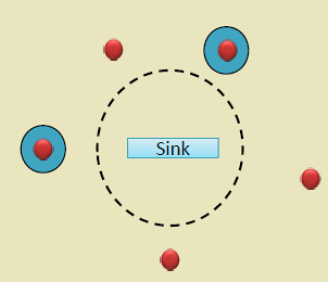
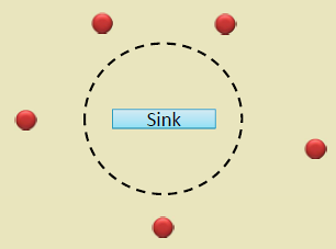
422.5 Mobile Sink (Mobile Base Station)
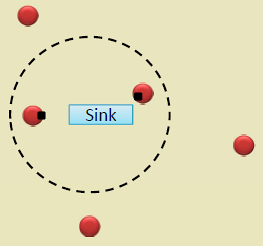


A mobile sink actively moves through the sensor field to collect data from stationary or mobile sensor nodes. This approach addresses the hotspot problem in stationary sink deployments.
Benefits:
- Distributes energy consumption evenly
- Increases network lifetime significantly (up to 5-10x)
- Reduces multi-hop communication overhead
- Balances traffic load
422.5.1 Path Planning Strategies
%% fig-alt: "Decision tree for mobile sink path planning showing three strategies: Random Walk (simple, unpredictable latency), Predefined Path (predictable, not adaptive), and Adaptive Path (optimized but complex computation)."
%%{init: {'theme': 'base', 'themeVariables': { 'primaryColor': '#2C3E50', 'primaryTextColor': '#fff', 'primaryBorderColor': '#16A085', 'lineColor': '#16A085', 'secondaryColor': '#E67E22', 'tertiaryColor': '#7F8C8D', 'fontSize': '16px'}}}%%
graph TD
    Strategy{Mobile Sink<br/>Path Planning}

    Strategy --> Random[Random Walk<br/>Unpredictable path]
    Strategy --> Predefined[Predefined Path<br/>Fixed route]
    Strategy --> Adaptive[Adaptive Path<br/>Based on data demand]

    Random --> R_Pro[Pro: Simple,<br/>Low overhead]
    Random --> R_Con[Con: Unpredictable<br/>latency]

    Predefined --> P_Pro[Pro: Predictable,<br/>Easy planning]
    Predefined --> P_Con[Con: Not adaptive]

    Adaptive --> A_Pro[Pro: Optimized<br/>collection]
    Adaptive --> A_Con[Con: Complex<br/>computation]

    style Strategy fill:#16A085,stroke:#2C3E50,color:#fff
    style Random fill:#E67E22,stroke:#16A085,color:#fff
    style Predefined fill:#E67E22,stroke:#16A085,color:#fff
    style Adaptive fill:#2C3E50,stroke:#16A085,color:#fff
    style A_Pro fill:#16A085,stroke:#2C3E50,color:#fff
Strategy Comparison:
| Strategy | Latency | Energy Balance | Complexity | Best For |
|---|---|---|---|---|
| Random Walk | Variable | Good (long-term) | Low | Simple deployments |
| Predefined | Predictable | Moderate | Low | Regular routes (buses) |
| Adaptive | Optimized | Excellent | High | Critical data collection |
422.6 Data MULEs (Mobile Ubiquitous LAN Extensions)
Data MULEs are mobile entities that physically transport data from sensors to the sink. Unlike mobile sinks that follow planned paths, MULEs often move based on existing mobility patterns (e.g., buses, animals, humans).
422.6.1 Operational Model
- Mobile entity (bus, animal, robot) moves through the sensor field
- Sensors detect MULE proximity and transmit buffered data
- MULE buffers collected data from multiple sensors
- MULE delivers aggregated data to sink when in range
- Process repeats with each MULE pass
%% fig-alt: "Sequence diagram showing Data MULE operation: Sensors buffer data, MULE moves into range of Sensor 1 and collects data, then Sensor 2, then delivers all collected data to Base Station."
%%{init: {'theme': 'base', 'themeVariables': { 'primaryColor': '#2C3E50', 'primaryTextColor': '#fff', 'primaryBorderColor': '#16A085', 'lineColor': '#16A085', 'secondaryColor': '#E67E22', 'tertiaryColor': '#7F8C8D', 'fontSize': '16px'}}}%%
sequenceDiagram
    participant S1 as Sensor 1
    participant S2 as Sensor 2
    participant MULE as Data MULE<br/>(Bus/Animal)
    participant Sink as Base Station

    Note over S1,S2: Sensors buffer data
    S1->>S1: Store measurements
    S2->>S2: Store measurements

    MULE->>S1: Move into range
    S1->>MULE: Upload buffered data
    Note over MULE: Store S1 data

    MULE->>S2: Move into range
    S2->>MULE: Upload buffered data
    Note over MULE: Store S2 data

    MULE->>Sink: Move into sink range
    MULE->>Sink: Upload all collected data
    Note over Sink: Process aggregated data
422.6.2 Real-World MULE Examples
ZebraNet (Kenya, 2004):
- 200 soil/vegetation sensors scattered across 50 km² savanna
- 30 zebras with GPS collars act as data MULEs
- Sensors buffer readings for days
- When zebra wanders within 50m, sensor wakes and uploads data
- Zebra stores data until visiting watering hole with base station
- Result: Zero mobility energy cost - zebra movement is free!
DakNet (India, 2003):
- Rural villages without internet connectivity
- Buses carry Wi-Fi access points as data MULEs
- Villagers upload/download data when bus passes
- Store-carry-forward email and web content
- Result: Internet access for remote communities at minimal cost
422.7 DTN Routing: Spray and Wait
For networks with intermittent connectivity, Delay-Tolerant Networking (DTN) protocols handle message delivery when end-to-end paths rarely exist.
Spray and Wait limits message replication to control overhead while maintaining good delivery probability.
422.7.1 Operation with L=6 Copies
Spray Phase:
- Source has L=6 message copies
- When encountering other nodes, transfer copies
- Binary spray: Split remaining copies (keep 3, give 3)
- Continue until all L copies distributed to different relay nodes
Wait Phase:
- Nodes with copies only forward to destination (direct delivery)
- No forwarding to other relay nodes
- Each holder “waits” to encounter destination directly
Performance Comparison:
| Protocol | Copies | Delivery Rate | Overhead |
|---|---|---|---|
| Epidemic | Unlimited | ~98% | 150x |
| Spray and Wait (L=6) | 6 | ~85% | 6x |
| Direct Delivery | 1 | ~40% | 1x |
422.8 Knowledge Check
422.9 Summary
This chapter covered the three key components of mobile wireless sensor networks:
- Mobile Sensor Nodes: Self-propelled or attached sensors using wheels, propellers, thrusters, or animal/human carriers, operating through sense-buffer-transfer cycles
- Mobile Sinks: Moving base stations that actively collect data using random walk, predefined, or adaptive path planning strategies
- Data MULEs: Mobile entities that leverage existing mobility (buses, animals, vehicles) for zero-cost store-carry-forward data collection
- DTN Routing: Spray and Wait and other protocols for intermittent connectivity, trading delivery guarantees for bounded overhead
422.10 What’s Next
The next chapter explores MWSN Types and Mobile Entities, examining underwater, terrestrial, and aerial mobile sensor networks, plus how humans, vehicles, and robots serve as mobile sensing platforms in daily life.