%% fig-alt: "Comparison of hop count routing (chooses 2-hop path with poor links) vs link quality routing (chooses 3-hop path with reliable links)"
%%{init: {'theme': 'base', 'themeVariables': {'primaryColor': '#2C3E50', 'primaryTextColor': '#fff', 'primaryBorderColor': '#16A085', 'lineColor': '#16A085', 'secondaryColor': '#E67E22', 'tertiaryColor': '#ECF0F1', 'fontSize': '16px'}}}%%
graph LR
    subgraph "Hop Count vs Link Quality Routing"
        SOURCE["Source<br/>Node"]

        PATH1_H1["Hop 1<br/>PDR: 50%"]
        PATH1_H2["Hop 2<br/>PDR: 50%"]

        PATH2_H1["Relay 1<br/>PDR: 90%"]
        PATH2_H2["Relay 2<br/>PDR: 90%"]
        PATH2_H3["Relay 3<br/>PDR: 90%"]

        SINK["Sink<br/>Node"]
    end

    SOURCE -->|"Path 1:<br/>2 hops"| PATH1_H1
    PATH1_H1 --> PATH1_H2
    PATH1_H2 --> SINK

    SOURCE -->|"Path 2:<br/>3 hops"| PATH2_H1
    PATH2_H1 --> PATH2_H2
    PATH2_H2 --> PATH2_H3
    PATH2_H3 --> SINK

    PATH1_H2 -.-> COST1["Expected TX:<br/>1/0.5 + 1/0.5<br/>= 4 transmissions"]
    PATH2_H3 -.-> COST2["Expected TX:<br/>1/0.9 × 3<br/>= 3.33 transmissions"]

    COST1 -.->|"Hop count chooses this"| BAD["Path 1: Higher cost<br/>More retransmissions"]
    COST2 -.->|"ETX chooses this"| GOOD["Path 2: Lower cost<br/>Better overall"]

    style SOURCE fill:#2C3E50,stroke:#16A085,stroke-width:3px,color:#fff
    style PATH1_H1 fill:#E74C3C,stroke:#2C3E50,stroke-width:2px,color:#fff
    style PATH1_H2 fill:#E74C3C,stroke:#2C3E50,stroke-width:2px,color:#fff
    style PATH2_H1 fill:#16A085,stroke:#2C3E50,stroke-width:2px,color:#fff
    style PATH2_H2 fill:#16A085,stroke:#2C3E50,stroke-width:2px,color:#fff
    style PATH2_H3 fill:#16A085,stroke:#2C3E50,stroke-width:2px,color:#fff
    style SINK fill:#E67E22,stroke:#2C3E50,stroke-width:3px,color:#fff
    style COST1 fill:#FADBD8,stroke:#E74C3C,stroke-width:2px
    style COST2 fill:#D5F4E6,stroke:#16A085,stroke-width:2px
    style BAD fill:#F5B7B1,stroke:#E74C3C,stroke-width:2px,color:#000
    style GOOD fill:#A9DFBF,stroke:#16A085,stroke-width:2px,color:#000
440 Link Quality Based Routing
440.1 Learning Objectives
By the end of this chapter, you will be able to:
- Evaluate Link Quality: Use link quality metrics to improve routing reliability and performance
- Implement WMEWMA: Configure Window Mean with Exponentially Weighted Moving Average for link estimation
- Calculate ETX/MIN-T: Compute Expected Transmission Count for path selection
- Avoid Gray Zone Links: Identify and route around unreliable intermediate-distance links
440.2 Prerequisites
Before diving into this chapter, you should be familiar with:
- WSN Routing Challenges: Understanding why hop count is insufficient for WSN routing
- Data Aggregation: How aggregation reduces transmissions and why reliable paths matter
- Wireless Sensor Networks: WSN radio characteristics and communication patterns
440.3 Introduction
Traditional routing protocols use hop count as the primary metric. However, in WSNs with unreliable wireless links, the shortest path may not be optimal.
440.4 Problems with Hop Count
440.4.1 1. Ignores Link Quality
A 3-hop path with reliable links is better than a 2-hop path with 50% loss: - Retransmissions on bad links waste energy - Total transmissions often higher on “shorter” paths
440.4.2 2. Doesn’t Account for Asymmetry
Forward and reverse links may have different quality: - Data might reach the next hop successfully - But ACKs fail on the poor reverse link - Results in unnecessary retransmissions
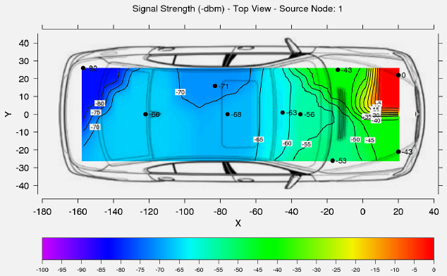
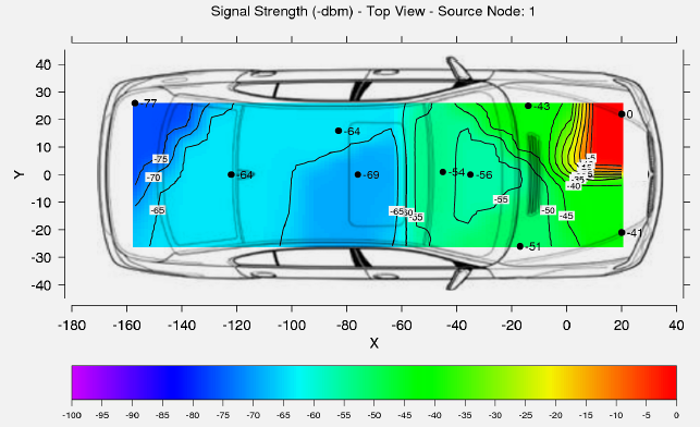
440.4.3 3. Assumes Spherical Communication Range
Reality shows highly irregular communication patterns: - Obstacles create dead zones - Interference varies by location - Fading effects unpredictable
440.5 RSSI (Received Signal Strength Indicator)
RSSI measures the power of a received radio signal. It provides a basic indication of link quality.
440.5.1 Characteristics
- Higher RSSI generally means better link quality
- Varies with distance, obstacles, interference
- Highly dynamic in mobile scenarios
- Can be measured passively
440.5.2 Limitations
- Temporal variations (fading)
- Spatial variations (multipath)
- Doesn’t directly indicate packet delivery rate
- Requires calibration for different hardware
440.6 Link Estimation with WMEWMA
NoteAcademic Resource: Cambridge Mobile and Sensor Systems
Source: University of Cambridge, Mobile and Sensor Systems Course (Prof. Cecilia Mascolo)
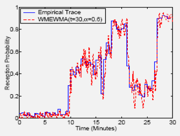
WMEWMA (Window Mean with Exponentially Weighted Moving Average) combines short-term and long-term link quality assessment.
440.6.1 Components
Snooping: Monitor broadcast packets from neighbors, track sequence numbers to detect losses
Window Mean (WM): Count packets received in recent window (e.g., last 30 packets)
EWMA: Exponentially weighted moving average smooths estimates over time
440.6.2 Formula
EWMA(t_x) = α × MA(t_x) + (1 - α) × EWMA(t_{x-1})Where: - MA(t_x): Number of packets received in window t_x - α ∈ (0, 1): Weight parameter (higher = more responsive) - Typical: α = 0.6, window = 30 packets
440.6.3 Why WMEWMA Works
The combination provides: - WM (Window Mean): Fast response to sudden link degradation - EWMA: Stability against transient fluctuations - Minimum of both: Conservative estimate that responds quickly to failures while filtering noise
440.7 MIN-T (Minimum Transmission) Metric
MIN-T estimates the expected number of transmissions required to successfully deliver a packet over a path, accounting for retransmissions.
440.7.1 Formula for Link Cost
Cost(link) = 1 / (P_forward × P_backward)Where: - P_forward: Forward link delivery probability - P_backward: Backward link delivery probability (for ACKs)
440.7.2 Path Cost
Cost(path) = Σ Cost(link_i) for all links in path440.7.3 Example Calculation
| Link | P_forward | P_backward | Cost |
|---|---|---|---|
| A→B | 0.9 | 0.9 | 1/(0.9×0.9) = 1.23 |
| B→C | 0.5 | 0.5 | 1/(0.5×0.5) = 4.0 |
Total path cost: 1.23 + 4.0 = 5.23 expected transmissions
440.8 ETX (Expected Transmission Count)
ETX is equivalent to MIN-T and is the standard metric used in many WSN protocols.
440.8.1 Calculation
ETX_link = 1 / (PRR_forward × PRR_reverse)
ETX_path = Σ ETX_link for all links
440.8.2 Path Comparison Example
| Path | Hops | Link PRRs | ETX per Link | Total ETX |
|---|---|---|---|---|
| A | 2 | 50%, 50% | 4.0, 4.0 | 8.0 |
| B | 3 | 90%, 90%, 90% | 1.23, 1.23, 1.23 | 3.69 |
Path B wins despite being longer (fewer expected transmissions = less energy).
440.9 Worked Example: ETX-Based Path Selection
NoteWorked Example: ETX-Based Routing Path Selection
Scenario: An industrial monitoring WSN tracks vibration levels on factory equipment. A sensor node S needs to route critical alarm data to the gateway G. Two candidate paths exist with different link qualities measured via probe packets.
Given:
| Path | Hops | Link Qualities (PRR) | Transmission Energy |
|---|---|---|---|
| Path A | 2 | S-R1: 95%, R1-G: 90% | 25 mJ per TX |
| Path B | 3 | S-R2: 85%, R2-R3: 80%, R3-G: 75% | 25 mJ per TX |
| Path C | 2 | S-R4: 60%, R4-G: 55% | 25 mJ per TX |
Steps:
Calculate ETX for each path (assuming symmetric links: ETX = 1/PRR²):
Path A ETX calculation:
- Link S-R1: ETX = 1 / (0.95 × 0.95) = 1 / 0.9025 = 1.11
- Link R1-G: ETX = 1 / (0.90 × 0.90) = 1 / 0.81 = 1.23
- Path A Total ETX = 1.11 + 1.23 = 2.34 transmissions
Path B ETX calculation:
- Link S-R2: ETX = 1 / (0.85)² = 1.38
- Link R2-R3: ETX = 1 / (0.80)² = 1.56
- Link R3-G: ETX = 1 / (0.75)² = 1.78
- Path B Total ETX = 1.38 + 1.56 + 1.78 = 4.72 transmissions
Path C ETX calculation (shortest by hop count):
- Link S-R4: ETX = 1 / (0.60)² = 2.78
- Link R4-G: ETX = 1 / (0.55)² = 3.31
- Path C Total ETX = 2.78 + 3.31 = 6.09 transmissions
Calculate expected energy consumption:
- Path A: 2.34 TX × 25 mJ = 58.5 mJ
- Path B: 4.72 TX × 25 mJ = 118.0 mJ
- Path C: 6.09 TX × 25 mJ = 152.3 mJ
Result:
| Metric | Path A (2 hops) | Path B (3 hops) | Path C (2 hops) |
|---|---|---|---|
| ETX | 2.34 (best) | 4.72 | 6.09 |
| Energy | 58.5 mJ (best) | 118.0 mJ | 152.3 mJ |
| First-attempt success | 85.5% | 51.0% | 33.0% |
Path A is optimal despite having the same hop count as Path C. The high link quality saves 93.8 mJ per packet (62% energy reduction) compared to Path C.
Key Insight: Hop-count routing would see Paths A and C as equivalent (both 2 hops), potentially selecting the inferior Path C. ETX-based routing correctly identifies that link quality dominates path selection.
440.10 Common Pitfalls
CautionPitfall: Choosing Shortest Path Without Link Quality Assessment
The Mistake: Implementing hop-count based routing in WSN deployments, assuming “fewer hops = better performance,” then experiencing 30-50% packet loss because the shortest path traverses marginal wireless links.
Why It Happens: Traditional networking education emphasizes shortest path algorithms (Dijkstra, Bellman-Ford). Teams apply this intuition without realizing that a “2-hop” path with 90% link quality outperforms a “1-hop” path with 50% link quality. Hop count ignores the retransmission cost of poor links.
The Fix: Use link quality metrics like ETX (Expected Transmission Count) or MIN-T instead of hop count:
- ETX = 1/(forward_delivery_rate × reverse_delivery_rate)
- A 3-hop path with ETX=3.3 beats a 2-hop path with ETX=8.0
- Measure link quality during network formation using probe packets
- Update metrics periodically to adapt to changing conditions
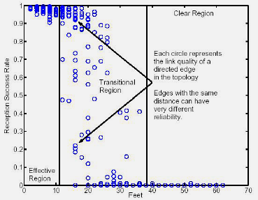
CautionPitfall: Gray Zone Links
The Problem: Links at intermediate distances (the “gray zone”) have highly variable quality: - Sometimes work (60% delivery) - Sometimes fail (30% delivery) - Unpredictable behavior
Why It Happens: At the edge of transmission range: - Signal strength varies with environmental conditions - Small movements cause large quality changes - Interference effects magnified
The Fix: - If measured PRR is between 10-90%, consider the link unreliable - Prefer links with PRR > 90% (clearly good) or < 10% (clearly avoid) - Use hysteresis: don’t switch routes for small quality differences - Require stable measurements over time (20+ packets minimum)
440.11 Knowledge Check
440.12 What’s Next?
Now that you understand link quality based routing, the next chapter explores the Trickle Algorithm for efficient network reprogramming and code dissemination.
Continue to Trickle Algorithm →
NoteRelated Chapters
- WSN Routing Fundamentals - Overview of WSN routing challenges and classification
- WSN Routing: Directed Diffusion - Data-centric routing with interests and gradients
- WSN Routing: Data Aggregation - In-network data processing techniques
- WSN Routing: Trickle Algorithm - Network reprogramming protocol
- WSN Routing: Labs and Games - Hands-on practice and interactive simulations