%% fig-alt: "Data aggregation architecture showing 100 sensors organized into 5 aggregation groups, reducing transmission from 100 to 5 messages at sink"
%%{init: {'theme': 'base', 'themeVariables': {'primaryColor': '#2C3E50', 'primaryTextColor': '#fff', 'primaryBorderColor': '#16A085', 'lineColor': '#16A085', 'secondaryColor': '#E67E22', 'tertiaryColor': '#ECF0F1', 'fontSize': '16px'}}}%%
graph TD
    subgraph "Data Aggregation in WSN"
        SENSORS["100 Sensor<br/>Nodes"]

        AGG1["Aggregator 1:<br/>20 readings<br/>→ 1 summary"]
        AGG2["Aggregator 2:<br/>20 readings<br/>→ 1 summary"]
        AGG3["Aggregator 3:<br/>20 readings<br/>→ 1 summary"]
        AGG4["Aggregator 4:<br/>20 readings<br/>→ 1 summary"]
        AGG5["Aggregator 5:<br/>20 readings<br/>→ 1 summary"]

        SINK["Sink:<br/>5 aggregates<br/>vs 100 raw"]
    end

    SENSORS -->|"Transmit raw data"| AGG1
    SENSORS -->|"Transmit raw data"| AGG2
    SENSORS -->|"Transmit raw data"| AGG3
    SENSORS -->|"Transmit raw data"| AGG4
    SENSORS -->|"Transmit raw data"| AGG5

    AGG1 -->|"Min/Max/Avg"| SINK
    AGG2 -->|"Min/Max/Avg"| SINK
    AGG3 -->|"Min/Max/Avg"| SINK
    AGG4 -->|"Min/Max/Avg"| SINK
    AGG5 -->|"Min/Max/Avg"| SINK

    SINK -.-> BENEFIT["Energy Savings:<br/>95% reduction<br/>in transmissions"]
    SINK -.-> TRADE["Trade-off:<br/>Information loss<br/>vs efficiency"]

    style SENSORS fill:#2C3E50,stroke:#16A085,stroke-width:3px,color:#fff
    style AGG1 fill:#16A085,stroke:#2C3E50,stroke-width:2px,color:#fff
    style AGG2 fill:#16A085,stroke:#2C3E50,stroke-width:2px,color:#fff
    style AGG3 fill:#16A085,stroke:#2C3E50,stroke-width:2px,color:#fff
    style AGG4 fill:#16A085,stroke:#2C3E50,stroke-width:2px,color:#fff
    style AGG5 fill:#16A085,stroke:#2C3E50,stroke-width:2px,color:#fff
    style SINK fill:#E67E22,stroke:#2C3E50,stroke-width:3px,color:#fff
    style BENEFIT fill:#D5F4E6,stroke:#16A085,stroke-width:2px
    style TRADE fill:#FADBD8,stroke:#E67E22,stroke-width:2px
439 Data Aggregation in WSN Routing
439.1 Learning Objectives
By the end of this chapter, you will be able to:
- Apply Data Aggregation: Implement in-network data processing to reduce communication overhead
- Select Aggregation Functions: Choose appropriate functions (MIN, MAX, AVG, SUM) for different applications
- Evaluate Aggregation Metrics: Measure accuracy, completeness, latency, and message overhead
- Design Aggregation Trees: Structure networks for efficient data combination
439.2 Prerequisites
Before diving into this chapter, you should be familiar with:
- Directed Diffusion: Understanding data-centric routing and gradient-based forwarding
- WSN Routing Challenges: Why energy efficiency is critical in sensor networks
- Wireless Sensor Networks: WSN architecture and multi-hop communication
439.3 Introduction
Data aggregation combines data from multiple sensors to reduce the number of transmissions, saving energy and bandwidth. This is one of the most effective energy-saving techniques in WSN routing.
439.4 Aggregation Benefits
439.4.1 Energy Savings
- Fewer transmissions = less energy consumed
- Particularly effective in dense networks
- Can extend network lifetime by 70-90%
439.4.2 Bandwidth Efficiency
- Reduces network congestion
- Lowers collision probability
- Improves delivery latency
439.4.3 Data Quality
- Averaging reduces noise
- Outlier detection and filtering
- Temporal and spatial correlation exploitation
439.5 Aggregation Functions
439.5.1 Simple Aggregation
| Function | Description | Use Case |
|---|---|---|
| MIN | Minimum value | Lowest temperature, closest distance |
| MAX | Maximum value | Peak temperature, farthest reading |
| SUM | Total of all values | Total rainfall, cumulative count |
| COUNT | Number of readings | Active nodes, detection events |
| AVERAGE | Mean value | Average temperature across region |
439.5.2 Statistical Aggregation
| Function | Description | Use Case |
|---|---|---|
| MEDIAN | Middle value | Robust central tendency |
| VARIANCE | Spread of values | Variability assessment |
| STANDARD DEVIATION | Measure of dispersion | Quality control bounds |
| HISTOGRAM | Distribution of values | Pattern analysis |
439.5.3 Duplicate-Sensitive Functions
| Function | Description | Use Case |
|---|---|---|
| DISTINCT COUNT | Count unique values | Unique detection events |
| SET UNION | Combine unique elements | Aggregate unique IDs |
439.5.4 Complex Queries
| Function | Description | Use Case |
|---|---|---|
| TOP-K | K largest/smallest values | Hot spots, anomalies |
| THRESHOLD | Values exceeding threshold | Alert generation |
| EVENT DETECTION | Specific patterns | Intrusion, fire detection |
439.6 Aggregation Metrics
439.6.1 1. Accuracy
Difference between aggregated result and true result:
Error = |Aggregated_Value - True_Value| / True_ValueFactors affecting accuracy: - Packet loss (missing readings) - Sensor calibration errors - Temporal misalignment
439.6.2 2. Completeness
Percentage of readings included in aggregate:
Completeness = Readings_Included / Total_ReadingsHigher completeness = more representative aggregate. Trade-off with latency (waiting for stragglers).
439.6.3 3. Latency
Time from sensing to sink reception:
- Aggregation introduces delay (waiting for multiple readings)
- Must balance freshness vs. completeness
- Application-dependent requirements
439.6.4 4. Message Overhead
Number of messages transmitted:
- Primary benefit of aggregation
- Measure: messages with vs. without aggregation
- Target: 60-95% reduction typical
439.7 Application-Appropriate Aggregation
CautionPitfall: Over-Aggregating Critical Data
The Mistake: Applying aggressive data aggregation (averaging, compression) uniformly across all sensor data, then missing critical events because anomalies were smoothed away by spatial averaging.
Why It Happens: Aggregation dramatically reduces energy consumption (95% savings possible), so teams maximize it. However, if 1 out of 20 sensors detects a fire while 19 report normal, the cluster average temperature may remain below the alarm threshold.
The Fix: Use aggregation functions appropriate to your application:
- For event detection: Use MAX or ANY-EXCEED-THRESHOLD instead of AVERAGE
- For anomaly detection: Forward individual readings that exceed thresholds
- Dual-path routing: Aggregated summaries for efficiency plus raw anomaly values on separate path
- Threshold-aware aggregation: Cluster heads forward individual readings that exceed critical thresholds, even when aggregating others
Example Decision Matrix:
| Application | Recommended Function | Rationale |
|---|---|---|
| Fire detection | MAX or THRESHOLD | Single hot spot must trigger alarm |
| Temperature monitoring | AVERAGE | Spatial average is meaningful |
| Intruder detection | ANY (boolean OR) | One detection = alert |
| Rainfall measurement | SUM | Total across region needed |
| Air quality | AVERAGE with outliers | Average, but flag anomalies |
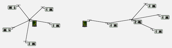
439.8 LEACH Clustering Demo
Explore how LEACH (Low-Energy Adaptive Clustering Hierarchy) balances energy consumption through randomized cluster head rotation. Watch energy depletion over multiple rounds and compare with direct transmission.
TipInteractive: LEACH Clustering Demo
How LEACH Works:
Cluster Head Election: Each round, nodes independently decide to become cluster heads (CH) based on probability
p. Nodes that were recently CH have lower probability, ensuring rotation.Cluster Formation: Non-CH nodes join the nearest cluster head to minimize transmission distance.
Data Aggregation: Members send data to their CH (short-distance, low energy). CHs aggregate data and transmit once to the sink (long-distance, high energy).
Energy Balancing: By rotating the CH role, no single node bears the aggregation burden throughout network lifetime.
Key Observations:
- Color gradient shows node energy levels (green=healthy, red=depleted)
- CH markers show current cluster heads and cluster regions
- Energy bars compare LEACH vs. direct transmission
- Run multiple rounds to see how CH role distributes and energy depletes evenly
Energy Comparison:
| Routing Method | Energy Profile |
|---|---|
| Direct Transmission | Nodes near sink deplete fast (hotspot) |
| Fixed Cluster Heads | CHs die quickly, others survive |
| LEACH (rotating) | Even depletion across all nodes |
Expected Energy Savings:
For a 100-node network with 10 clusters: - Direct: 100 long-distance transmissions - LEACH: 100 short + 10 long transmissions - Savings: 40-60% depending on topology
CautionPitfall: Fixed Cluster Head Selection
The Mistake: Designating cluster heads based on initial battery levels or geographic position, then having the network partition when all cluster heads die simultaneously while regular nodes still have 70% battery.
Why It Happens: Fixed cluster heads seem logical - “put the strongest nodes in charge.” But cluster heads consume 3-5x more energy than regular nodes due to receiving from members, aggregation, and long-range transmission to the sink. Static assignment concentrates this drain on a few nodes.
The Fix: Implement cluster head rotation as in LEACH:
- Each round, cluster heads are selected probabilistically
- Every node serves approximately equal time as CH over network lifetime
- Consider energy-weighted probability: nodes with more remaining energy have slightly higher CH probability
- Monitor CH energy levels and trigger early rotation if a CH drops below 20% while others have 50%+
439.9 Worked Example: LEACH Energy Analysis
NoteWorked Example: LEACH Cluster Head Selection and Energy Analysis
Scenario: A precision agriculture deployment monitors soil moisture across a 500m × 500m vineyard. The WSN uses LEACH protocol with 100 sensor nodes reporting to a base station located at coordinate (250m, 0m) at the vineyard edge.
Given:
| Parameter | Value |
|---|---|
| Total nodes | 100 |
| Initial energy per node | 2 J (Joules) |
| Cluster head probability (p) | 10% (0.1) |
| Energy for transmission (E_tx) | 50 nJ/bit |
| Energy for receiving (E_rx) | 50 nJ/bit |
| Energy for data aggregation | 5 nJ/bit/signal |
| Amplifier energy (E_amp) | 100 pJ/bit/m^2 |
| Data packet size | 4000 bits |
| Average distance to base station | 200 m |
| Average intra-cluster distance | 35 m |
Steps:
- Calculate expected cluster heads per round:
- Expected CHs = n × p = 100 × 0.1 = 10 cluster heads
- Average cluster size = 100 / 10 = 10 nodes per cluster (9 members + 1 CH)
- Calculate energy consumption for a regular node (cluster member):
- Transmit to CH (short range): E_member = E_tx × k + E_amp × k × d²
- E_member = (50 nJ/bit × 4000 bits) + (100 pJ/bit/m² × 4000 bits × 35² m²)
- E_member = 200 µJ + 490 µJ = 690 µJ per round
- Calculate energy consumption for a cluster head:
- Receive from 9 members: E_rx_total = 9 × E_rx × k = 9 × 50 nJ/bit × 4000 bits = 1,800 µJ
- Aggregate 10 signals: E_agg = 10 × 5 nJ/bit/signal × 4000 bits = 200 µJ
- Transmit to base station (long range): E_tx_bs = E_tx × k + E_amp × k × d²
- E_tx_bs = (50 nJ/bit × 4000 bits) + (100 pJ/bit/m² × 4000 bits × 200² m²)
- E_tx_bs = 200 µJ + 16,000 µJ = 16,200 µJ
- Total CH energy = 1,800 + 200 + 16,200 = 18,200 µJ per round
- Calculate network energy per round:
- 90 members × 690 µJ = 62,100 µJ
- 10 CHs × 18,200 µJ = 182,000 µJ
- Total network energy = 244,100 µJ = 244.1 mJ per round
- Estimate network lifetime:
- Total initial energy = 100 nodes × 2 J = 200 J
- Rounds until first node dies: ~200 J / 244.1 mJ = ~820 rounds
- With CH rotation, energy depletes evenly, extending usable lifetime
Result: With LEACH and p=0.1, the network consumes 244.1 mJ per data collection round. Cluster heads consume 26× more energy than members (18,200 µJ vs 690 µJ), which is why rotation is critical. Without rotation, the 10 static CHs would die in ~110 rounds while other nodes retain 94% energy.
Key Insight: The LEACH probability p=0.1 creates 10 clusters optimized for this 100-node network. Increasing p to 0.2 would create 20 smaller clusters with shorter intra-cluster distances (less member energy) but more long-range CH-to-base transmissions (more total CH energy). For deployments where base station distance dominates, lower p values (larger clusters, fewer CHs) are more energy-efficient.
439.10 Knowledge Check
439.11 What’s Next?
Now that you understand data aggregation techniques, the next chapter explores Link Quality Based Routing, which uses metrics like ETX and RSSI to select reliable paths.
Continue to Link Quality Routing →
NoteRelated Chapters
- WSN Routing Fundamentals - Overview of WSN routing challenges and classification
- WSN Routing: Directed Diffusion - Data-centric routing with interests and gradients
- WSN Routing: Link Quality - RSSI, WMEWMA, and MIN-T metrics
- WSN Routing: Trickle Algorithm - Network reprogramming protocol
- WSN Routing: Labs and Games - Hands-on practice and interactive simulations