Energy is the most critical resource in battery-powered WSNs, fundamentally limiting network lifetime and capabilities. Effective energy management is essential for practical deployments.
367.1.1 Energy Consumption Profile
Radio Communication (Dominant Consumer): - Transmission: 10-50 mW typical - Reception: 10-40 mW (often comparable to transmission) - Idle listening: 1-20 mW (significant waste in low-traffic networks)
Processing: - Active computation: 1-10 mW - Sleep mode: 1-100 μW - Deep sleep: < 1 μW
Memory Access: - Flash write operations: High energy cost - RAM access: Relatively low cost
367.1.2 Energy Conservation Strategies
Duty Cycling: Alternating between active and sleep periods to reduce average power consumption.
Approaches: - Time-based: Fixed sleep/wake schedules - Event-driven: Wake on external interrupts (sensors, messages) - Demand-driven: Wake based on predicted activity or queries
Challenges: - Latency increase due to sleep periods - Synchronization for communication - Balancing energy savings vs. responsiveness
Data Reduction: Minimizing amount of data transmitted to reduce communication energy.
Techniques: - Local processing and filtering - Data compression - In-network aggregation - Adaptive sampling rates - Threshold-based reporting (only significant changes)
Topology Control: Managing network topology to optimize energy consumption.
Methods: - Transmission power adjustment - Reducing node degree (number of neighbors) - Clustering and hierarchy formation - Sleep scheduling coordination
Routing Optimization: Selecting energy-efficient paths for data delivery.
Strategies: - Minimum energy routing - Load balancing to avoid hotspots - Geographic routing to minimize hops - Multi-path routing for reliability
367.2 Distributed Coordination: Lessons from Nature
In 1986, computer scientist Craig Reynolds discovered something profound: complex swarm behavior—like flocking birds or schooling fish—emerges from just three simple local rules. No central controller, no global map, no leader. Each individual (“boid”) follows basic rules based only on nearby neighbors, yet the group achieves remarkable coordination.
This insight revolutionized distributed systems thinking and directly applies to WSN design: simple local rules → complex global behavior.
Figure 367.2: Diagram showing how separation, alignment, and cohesion rules lead to emergent network behaviors in WSN: optimal coverage, coordinated tracking, an…
TipKey Insight: The Power of Emergent Behavior
No central controller needed! Each sensor node follows simple local rules based only on nearby neighbors, yet the network achieves global objectives:
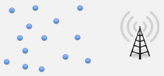
Coverage: Separation spreads nodes across the monitoring area, avoiding redundant overlap
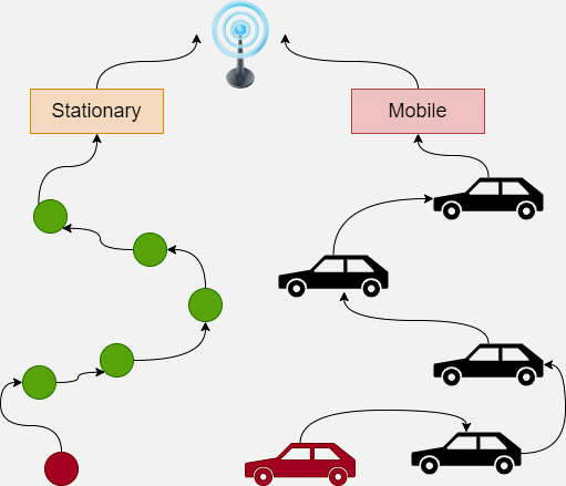
Tracking: Alignment coordinates pursuit of mobile targets (vehicles, wildlife) without centralized planning
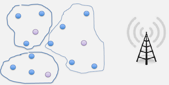
Connectivity: Cohesion prevents network fragmentation by maintaining neighbor links
This is the fundamental principle of emergent behavior in distributed systems: simple local interactions produce complex global patterns.
Why This Matters for WSN: - Scalability: Works with 10 nodes or 10,000 nodes (no central bottleneck) - Robustness: Network adapts to node failures automatically - Energy efficiency: No expensive global coordination messages - Self-organization: Network reconfigures as topology changes
Real-World Example: The PEGASIS (Power-Efficient GAthering in Sensor Information Systems) protocol uses alignment principles—nodes self-organize into a chain structure based only on neighbor distances, achieving optimal energy distribution without centralized planning.
Energy Harvesting: Supplementing battery power with ambient energy sources.
Sources: - Solar (outdoor deployments) - Vibration (machinery, bridges) - Thermal (temperature gradients) - RF energy harvesting - Wind or water flow
Challenges: - Intermittent availability - Energy storage requirements - Harvester efficiency - Cost and size constraints
WarningMesh Networks Aren’t Always the Answer
Developers often default to mesh topologies assuming “more paths = better reliability,” but mesh networks introduce significant energy and complexity costs. Each node must maintain routing tables, handle relayed traffic from neighbors (consuming energy), and suffer from the broadcast storm problem where route discovery floods propagate through the network. For many applications, simpler star or tree topologies with strategic gateway placement provide 90% of mesh benefits at 10% of the energy cost and complexity. Use mesh only when deployment area genuinely requires multi-hop communication beyond gateway range, or when mobility and dynamic topology changes are frequent. Consider hybrid approaches: mesh backbone with star clusters, providing scalability without universal mesh overhead.
WarningCommon Misconception: “The Hotspot Problem Will Solve Itself”
Myth: “If I deploy enough sensor nodes with redundant paths, the network will automatically balance energy consumption and nodes will all die around the same time.”
Reality: In multi-hop WSNs, nodes near the sink (gateway) become unavoidable “hotspots” that relay traffic from ALL downstream nodes, causing them to drain batteries 5-100× faster than edge nodes:
Edge node (far from gateway): Transmits only its own data (1 packet/minute → 2-year lifetime)
Hotspot node (near gateway): Relays own data + forwards 10-50 other nodes (50 packets/minute → 2-month lifetime)
Network failure: When hotspot nodes die, entire network partitions despite edge nodes having 95%+ battery
Real Example: Agricultural WSN with 100 sensors. Nodes closest to gateway died after 4 months, disconnecting 60 downstream sensors. Farmer lost $15,000 in crop yield due to undetected irrigation failure.
Solutions: 1. Multiple sinks: Deploy 3 strategically placed gateways to distribute relay load (3-month → 2-year lifetime) 2. Solar cluster heads: Use mains/solar-powered relay nodes in hotspot zones 3. Energy-aware routing: Route traffic around low-battery nodes (LEACH protocol) 4. Battery monitoring: Track battery levels remotely for predictive replacement
Figure 367.4: LEACH protocol operation showing cluster head selection and data aggregation
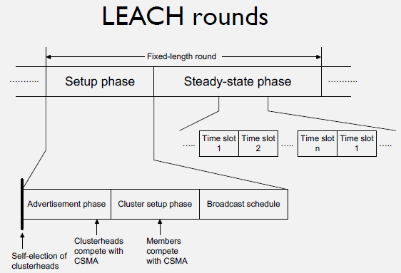
Figure 367.5: LEACH protocol rounds showing setup phase and steady-state data transmission phases
Figure 367.6: Multi-hop routing path in WSN showing data forwarding from source to sink through intermediate nodes
MAC Protocols: Coordinating medium access to minimize idle listening and collisions.
Examples: - S-MAC (Sensor-MAC): Coordinated sleep schedules - B-MAC (Berkeley MAC): Low-power listening with preambles - RI-MAC: Receiver-initiated communication - IEEE 802.15.4: CSMA/CA with optional beacon mode
Routing Protocols: Energy-aware path selection and load distribution.
Examples: - LEACH (Low-Energy Adaptive Clustering Hierarchy): Randomized cluster head rotation - PEGASIS (Power-Efficient GAthering in Sensor Information Systems): Chain-based routing - TEEN (Threshold sensitive Energy Efficient sensor Network): Event-driven reporting - Geographic routing: Position-based forwarding
367.3 Radio Duty Cycling
⏱️ ~12 min | ⭐⭐⭐ Advanced | 📋 P05.C25.U07
Radio duty cycling is one of the most effective energy conservation techniques in WSNs, reducing the time transceivers spend in energy-consuming states.
367.3.1 Duty Cycling Fundamentals
Duty Cycle Definition: The fraction of time a node’s radio is active (transmitting, receiving, or listening).
Example: A node awake 10ms every 100ms has a 10% duty cycle.
Impact: Reducing duty cycle from 100% to 1% can extend battery lifetime by 10-100x, depending on the relative power consumption of radio vs. other components.
367.3.2 Duty Cycling Approaches
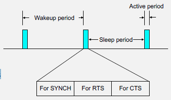
Synchronous Duty Cycling: Nodes coordinate wake/sleep schedules to ensure communication opportunities.
Characteristics: - Nodes wake up simultaneously - Requires clock synchronization - Lower latency for multi-hop communication - Examples: S-MAC, T-MAC
Figure 367.7: S-MAC protocol - synchronous duty cycling with coordinated sleep schedules for WSN energy conservation
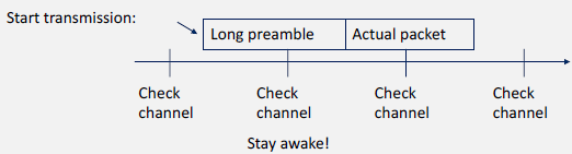
Figure 367.8: Preamble sampling mechanism for asynchronous duty cycling - sender transmits long preamble until receiver wakes
Advantages: - Predictable communication windows - Efficient for scheduled traffic - Coordinated network operation
Challenges: - Synchronization overhead and drift - Global schedule may not suit all nodes - Less flexibility for event-driven traffic
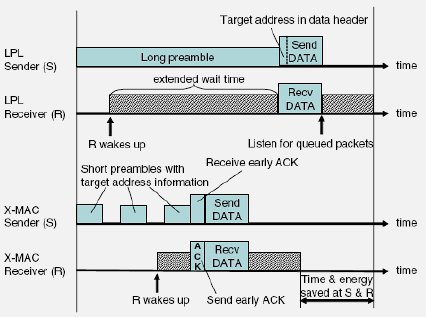
Asynchronous Duty Cycling: Nodes operate on independent schedules without global synchronization.
Characteristics: - No synchronization required - Senders must account for receiver schedules - Examples: B-MAC, X-MAC, RI-MAC
Figure 367.9: X-MAC protocol - asynchronous duty cycling with short preambles and early acknowledgment for energy efficiency
Mechanisms: - Preamble sampling: Sender transmits long preamble until receiver wakes - Wake-up beacons: Receivers announce availability - Receiver-initiated: Receivers poll for pending messages
Advantages: - No synchronization overhead - Flexible and adaptive - Supports mobile and heterogeneous networks
Challenges: - Potential latency increase - Energy cost of preambles or polling - Variable message delivery time
Hybrid Approaches: Combining synchronous and asynchronous techniques.
Examples: - Local synchronization within clusters, asynchronous between clusters - Schedule-based for regular traffic, on-demand for events - Adaptive switching based on traffic patterns
367.3.3 Advanced Duty Cycling Techniques
Adaptive Duty Cycling: Dynamically adjusting duty cycle based on conditions.
Parameters: - Traffic load (increase cycle during high activity) - Residual energy (reduce cycle when battery low) - Time of day (circadian patterns in environmental monitoring) - Event detection (increase sampling rate during events)
Predictive Duty Cycling: Using historical data and prediction models to optimize schedules.
Approaches: - Machine learning to predict traffic patterns - Correlation-based sensing (sensors with correlated readings coordinate) - Event prediction to pre-activate relevant nodes
Hierarchical Duty Cycling: Different duty cycles for different node roles.
Structure: - Cluster heads: Higher duty cycle for availability - Regular nodes: Lower duty cycle for energy conservation - Gateway nodes: Always-on or high duty cycle
Wake-on-Radio: Special low-power radio listens continuously, waking main radio when messages arrive.
Characteristics: - Main radio sleeps indefinitely - Wake-up radio consumes micro-watts - Triggered wake-up for main radio - Ultra-low average power consumption
Technologies: - Dedicated wake-up receivers - Ultra-low-power always-on circuits - RF energy harvesting for wake-up
367.3.4 Performance Trade-offs
Energy vs. Latency: Lower duty cycles save energy but increase message delivery latency.
Mitigation: - Multi-hop forwarding during wake periods - Predictive wake-up for urgent messages - Adaptive cycles based on message priority
Energy vs. Reliability: Sleeping nodes may miss messages or events.
Energy vs. Throughput: Limited active time constrains data transmission capacity.
Balancing: - Efficient data aggregation and compression - Adaptive duty cycle during high-traffic periods - Buffering and batch transmission - Priority-based scheduling
367.4 Production Framework: Complete WSN Management Platform
⏱️ ~10 min | ⭐⭐⭐ Advanced | 📋 P05.C25.U08
Below is a comprehensive Python framework for deploying and managing wireless sensor networks with node simulation, routing protocols, energy optimization, and network analytics.
NoteQuiz 2: Complete WSN Management Platform
Question 1: A WSN deployment uses sensor nodes with radios consuming 15 mA in idle listening mode and 20 mA during transmission. Each node has a 2000 mAh battery and transmits for 1% of the time. Without duty cycling (radio always on in idle mode), how long will the battery last?
💡 Explanation: Battery life = 2000 mAh / 15 mA = 133 hours = 5.5 days. This demonstrates why idle listening is so problematic - the radio consumes 15 mA continuously even when not transmitting. Many developers underestimate this: idle listening (15 mA) is nearly as expensive as active transmission (20 mA)! With 1% duty cycle and proper sleep modes (1 µA), the same battery would last: (0.01 × 20 mA + 0.99 × 0.001 mA) ≈ 0.2 mA average → 2000/0.2 = 10,000 hours = 416 days. Real-world impact: An agricultural WSN that fails after a week vs. one lasting over a year - the only difference is aggressive duty cycling. Solutions: synchronized sleep schedules (S-MAC), preamble sampling (B-MAC), or wake-up radios consuming microamps.
Question 2: In a 100-node WSN with a single sink node, nodes near the sink deplete their batteries 50x faster than edge nodes. After 3 months, these “hotspot” nodes die while edge nodes still have 95% battery remaining. What is the most effective solution?
💡 Explanation: Multiple sinks solve the hotspot problem by distributing relay traffic. With 3 sinks, each hotspot zone handles ~33% of traffic instead of 100%, extending lifetime from 3 months to potentially 2+ years. Why other options fail: (A) Higher transmission power increases energy consumption for ALL nodes, doesn’t address unequal load distribution. (B) Battery replacement is impractical for large deployments, especially in remote/inaccessible locations. (D) Reducing duty cycle helps but doesn’t solve the fundamental imbalance - hotspots still relay 50x more packets. Additional strategies: Mobile sinks that relocate periodically, energy-aware routing that avoids low-battery nodes, or overprovision hotspot zones with mains-powered relay nodes. Real example: 100-node agricultural WSN extended lifetime from 3 months to 2+ years by deploying 3 sinks instead of 1. The hotspot problem is the #1 cause of premature WSN failure.
Question 3: A smart agriculture WSN covers 1 km² with 200 sensor nodes. The development team proposes a full mesh topology where every node maintains routing to every other node. What is the primary concern with this approach?
💡 Explanation: Full mesh networks impose severe energy and complexity costs: (1) Routing overhead: Each node maintains tables for 199 neighbors, consuming memory and processing. (2) Relay traffic: Nodes must forward packets for neighbors, draining batteries even when not sensing. (3) Broadcast storms: Route discovery messages flood the network, consuming bandwidth and energy. (4) Complexity: Mesh protocols (AODV, DSR) are complex to implement and debug. For many applications, simpler topologies provide 90% of benefits at 10% of cost: Star topology with strategic gateway placement, tree topology with cluster heads, or hybrid approach (mesh backbone + star clusters). Use mesh only when: deployment genuinely requires multi-hop beyond gateway range, mobility requires dynamic topology changes, or critical redundancy justifies the cost. Real case: Agricultural WSN switched from full mesh to clustered star, reducing energy consumption by 70% while maintaining 95% coverage.
Question 4: A WSN monitoring system aggregates temperature data from 100 sensor nodes. Without aggregation, each node sends 10 bytes every minute to the sink (100 nodes × 10 bytes = 1000 bytes/min). With in-network aggregation at 5 cluster heads, what is the approximate data reduction?
💡 Explanation: With in-network aggregation: 100 nodes organized into 5 clusters of 20 nodes each. Each cluster head receives 20 readings but transmits only aggregated statistics (min/max/avg/count = ~40 bytes) instead of forwarding all 200 bytes. Total traffic: 5 clusters × 40 bytes = 200 bytes vs. 1000 bytes without aggregation = 80% reduction. Benefits beyond bandwidth: (1) Energy savings: Transmitting is expensive (20 mA), reducing transmissions from 100 to 5 saves massive energy. (2) Reduced collisions: Fewer simultaneous transmissions in shared wireless medium. (3) Better insights: Aggregate statistics (spatial averages, trends) often more useful than raw readings. (4) Scalability: Enables larger networks without overwhelming sink capacity. Trade-offs: Requires cluster head selection algorithms, aggregation delay for collecting readings, and cluster heads consume more energy (must stay awake to receive). Real-world: Environmental monitoring WSN extended lifetime from 6 months to 3 years using hierarchical aggregation.
Question 5: A WSN uses synchronized sleep scheduling (S-MAC) where nodes sleep 90% of the time and wake simultaneously every 1 second to communicate. A critical event occurs that requires immediate notification. What is the maximum notification delay?
💡 Explanation: With synchronized sleep (S-MAC), nodes wake together every 1 second. If an event occurs right after nodes sleep, the detecting node must wait up to 1 second until the next wake cycle to transmit. This is the fundamental latency vs. energy trade-off in duty-cycled WSNs. Improving response time: (1) Increase duty cycle: Wake every 0.1s (10% → 90% energy cost), (2) Adaptive listening: Stay awake longer after receiving packet (T-MAC), (3) Event-driven wake-up: Use low-power wake-up radios that monitor continuously while main radio sleeps (~10 µA vs. 15 mA), (4) Asynchronous protocols: Preamble sampling (B-MAC, X-MAC) allows anytime transmission with longer preambles. Application implications: Fire detection system with 1-second delay is acceptable, but gas leak detection may require faster response (use wake-up radios or higher duty cycle near hazardous areas). Real design: Mine safety monitoring uses 10% duty cycle in normal areas, 50% near hazards, and continuous wake-up radio monitoring for critical gas sensors.
Question 8: A precision agriculture WSN monitors soil moisture using 100 nodes. The system uses data aggregation where sensor readings are combined at intermediate nodes before transmission to the sink. Which aggregation function would be LEAST useful for irrigation decision-making?
💡 Explanation: SUM is least useful because it provides total moisture across all 100 sensors, which lacks meaningful agricultural context. What matters: spatial distribution (where is it dry?), statistical measures (average moisture), and extremes (driest/wettest areas). Useful aggregation functions: (1) MIN: Identifies critical dry zones needing immediate irrigation. Example: Field average is 60% but MIN is 20% → one zone needs water. (2) MAX: Finds oversaturated areas where irrigation should stop (prevents root rot, runoff). (3) MEAN: Overall field moisture guides general irrigation scheduling. (4) VARIANCE/STDDEV: Measures moisture uniformity - high variance indicates uneven irrigation requiring system adjustment. (5) SPATIAL AGGREGATION: Cluster-level averages (northwest quadrant = 45%, southeast = 65%) enable zone-specific irrigation. Advanced techniques: Suppress redundant transmissions when values haven’t changed significantly, transmit only anomalies (moisture drops >10%), or adaptive sampling (measure more frequently when moisture is near critical thresholds). Real system: Precision agriculture WSN reduced water usage by 40% using spatial MIN/MAX aggregation to target irrigation only where needed.
Question 11: A structural health monitoring WSN on a bridge uses accelerometer sensors to detect vibrations. The system must distinguish between normal traffic vibrations and dangerous structural oscillations. Which WSN characteristic is most critical?
💡 Explanation: Structural health monitoring requires coordinated vibration analysis across multiple sensor locations to distinguish vibration modes and identify structural issues. Critical requirements: (1) High sampling rates: Accelerometers must capture vibrations at 100-1000 Hz (vs. typical WSN’s 1 sample/min for temperature). (2) Time synchronization: Nodes must timestamp readings within microseconds to correlate vibrations across bridge spans. Without sync, cannot determine if vibration mode is torsional twist (dangerous) vs. vertical bounce (normal). (3) Data quality: 12-16 bit ADC resolution to capture subtle changes in vibration amplitude/frequency. (4) Reliable delivery: Lost vibration samples create gaps in analysis. Energy implications: High sampling rates and continuous operation require mains power or energy harvesting - pure battery operation is often infeasible. Comparison to other WSN applications: Agriculture monitoring (1 sample/min, loose timing, simple sensors) vs. structural health (100-1000 samples/sec, tight sync, complex analysis). Architecture: Often hybrid - continuous monitoring with local processing (FFT, anomaly detection) and selective cloud upload of events rather than raw data streams. Real deployment: Golden Gate Bridge uses 64 synchronized accelerometers with GPS time synchronization (±10 µs) for modal analysis.
Question 12: A wildlife tracking WSN deploys collar sensors on migrating animals. The network must operate for 2 years without maintenance. Which characteristic dominates the design?
💡 Explanation: Wildlife tracking WSNs face extreme energy constraints - collars are small, battery replacement requires recapturing animals (often impossible), and operation must span migration cycles (months to years). Energy optimization strategies: (1) Aggressive duty cycling: GPS active only 5 minutes/day instead of continuous (GPS consumes 50-100 mW). Sample location every few hours unless movement detected. (2) Event-driven operation: Accelerometer detects movement → activate GPS for tracking. Stationary periods → deep sleep (1 µA). (3) Scheduled uploads: Buffer location data and upload when near base stations instead of continuous transmission. (4) Adaptive sampling: Increase sampling rate during active periods (migration), decrease during rest periods. (5) Energy harvesting: Solar panels on collars (where feasible) extend operation indefinitely. Why other options don’t work: (A) Second-by-second updates drain batteries in days. (B) Wildlife moves - can’t deploy fixed infrastructure everywhere. (D) Animals spread across vast areas beyond multi-hop range; satellite/cellular more practical than mesh. Real example: Elephant collar tracking uses GPS sampling every 2 hours during day, every 6 hours at night, uploads via cellular when signal available. Battery life: 2-3 years on 10,000 mAh despite crossing thousands of kilometers.
Question 13: In a WSN using hierarchical clustering with cluster heads, why might cluster heads have shorter lifetimes than regular nodes?
💡 Explanation: Cluster heads have asymmetric energy consumption vs. regular nodes: (1) Receive duty: Must stay awake to receive data from all cluster members (20 nodes × 1s = 20s awake vs. 1s for regular nodes). (2) Aggregation processing: Compute statistics (min/max/avg) from received data. (3) Longer transmissions: Forwarding aggregated data to sink may be multi-hop with greater distance/power. (4) Coordination overhead: Broadcasting cluster schedule, handling member joins/leaves. Energy comparison: Regular node: sense (1s) + transmit (0.1s) + sleep. Cluster head: receive from members (20s) + aggregate (0.5s) + transmit to sink (0.2s) + sleep. Even with aggregation reducing transmission data, cluster heads consume 3-5x more energy. Solution: Rotate cluster head role (LEACH protocol): Every round, randomly select different nodes as cluster heads, distributing energy burden across all nodes. Example: Without rotation, cluster heads die in 3 months while members last 12 months → network fails early. With rotation, all nodes last ~10 months and network maintains coverage. Alternative: Deploy dedicated mains-powered or high-capacity battery cluster heads (more expensive but eliminates rotation overhead).
Question 14: A WSN uses gradient-based routing where each node knows its distance (hop count) to the sink and forwards packets to neighbors with smaller distance. A routing loop occurs where packets circulate indefinitely. What is the most likely cause?
💡 Explanation: Routing loops in gradient-based routing occur when gradient information becomes stale or inconsistent. Scenario: (1) Initially: Sink floods network establishing gradient (Sink=0, neighbors=1, their neighbors=2, etc.). (2) Node A (gradient=5) forwards to Node B (gradient=4) successfully. (3) Node B fails or link quality degrades. (4) Node B mistakenly advertises gradient=6 (incorrectly calculated due to loss of better path). (5) Loop forms: A (gradient=5) → B (gradient=6) → C (gradient=5) → A. Packet circulates indefinitely. Prevention mechanisms: (1) Periodic gradient refresh: Sink periodically re-floods network updating all gradients. (2) Sequence numbers: Detect and drop duplicate packets that have already been seen. (3) TTL (Time-To-Live): Decrement hop counter, drop when reaching zero to kill looped packets. (4) Multiple metrics: Combine gradient with link quality, energy levels to avoid failing paths. (5) Loop detection: Nodes track recently forwarded packets, detect circulation. Why important: Loops waste massive energy (packet retransmitted continuously) and prevent data delivery. Real incident: Environmental monitoring WSN experienced 3-day routing loop consuming 40% of network energy before loop detection mechanism activated.
Question 15: A WSN application developer must choose between event-driven sensing (nodes transmit only when detecting events) and periodic sensing (nodes transmit every 60 seconds). For monitoring rare events like equipment failures occurring every few days, which approach provides better energy efficiency and why?
💡 Explanation: Event-driven sensing provides massive energy savings for rare events: (1) Deep sleep: Nodes sleep (1 µA) except for brief wake-ups to check sensor or respond to interrupts. (2) Transmission only on events: If events occur every 3 days, nodes transmit 120 times/year instead of 525,600 times/year (every 60s). (3) Energy calculation: Event-driven: 99.99% sleep (1 µA) + 0.01% event handling (20 mA average) ≈ 2 µA average. Periodic: 0.1% active (60s sampling/transmission every hour, 20 mA) + 99.9% sleep (1 µA) ≈ 20 µA average. 10x energy savings!Implementation: Use interrupt-driven sensing (accelerometer interrupt on vibration, PIR interrupt on motion) rather than polling. Node stays in deep sleep until hardware interrupt triggers wake-up. Trade-off: Event detection latency. If using polling (wake every 10s to check sensor), might miss 9.9s of event. Solution: Use analog comparators or dedicated low-power event detectors that monitor continuously while CPU sleeps. Real application: Pipeline leak detection using acoustic sensors. Event-driven approach: 5-year battery life. Periodic sampling: 6-month battery life. The difference between practical deployment and frequent maintenance.