365  WSN Coverage Types

NoteKey Concepts

• Area Coverage: Monitoring every point in a continuous 2D region with sensor coverage
• Point Coverage: Monitoring discrete critical locations (doors, valves, junctions)
• Barrier Coverage: Detecting intruders crossing a border or perimeter
• K-Coverage: Redundancy where every point is covered by at least k sensors
• Weak vs Strong Barrier: Path-intersection detection vs continuous path monitoring

365.1 Learning Objectives

By the end of this chapter, you will be able to:

• Differentiate Coverage Types: Distinguish area, point, and barrier coverage applications
• Calculate Sensor Requirements: Compute minimum sensors for each coverage type
• Design K-Coverage Systems: Select appropriate redundancy levels for fault tolerance
• Choose Barrier Strategies: Decide between weak and strong barrier coverage based on requirements

TipMVU: Minimum Viable Understanding

Core concept: Coverage problems fall into three categories: area (monitor continuous region), point (monitor discrete locations), and barrier (detect crossings). Why it matters: Choosing the wrong coverage type wastes sensors - area coverage for sparse valve monitoring costs 5-10x more than point coverage. Key takeaway: Match coverage type to application: area for environmental monitoring, point for infrastructure, barrier for security.

365.2 Prerequisites

Before diving into this chapter, you should be familiar with:

• WSN Coverage Fundamentals: Understanding of coverage definitions, connectivity, and deployment strategies
• Sensor Fundamentals and Types: Knowledge of sensing range characteristics

NoteRelated Chapters

Fundamentals: - WSN Coverage Fundamentals - Coverage basics and connectivity

Algorithms: - WSN Coverage Algorithms - OGDC and coverage maintenance

Implementations: - WSN Coverage Implementations - Hands-on labs and Python code

Review: - WSN Coverage Review - Comprehensive coverage quiz and summary

365.3 Coverage Problem Types

~15 min | Intermediate | P05.C29.U02

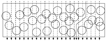
365.3.1 Area Coverage

Objective: Monitor every point in a continuous 2D region.

%% fig-alt: "Area coverage model showing how multiple sensor coverage areas combine to cover monitored region, with complete coverage or coverage holes outcome"
%%{init: {'theme': 'base', 'themeVariables': {'primaryColor': '#2C3E50', 'primaryTextColor': '#fff', 'primaryBorderColor': '#16A085', 'lineColor': '#16A085', 'secondaryColor': '#E67E22', 'tertiaryColor': '#ECF0F1', 'fontSize': '16px'}}}%%
graph TD
    subgraph "Area Coverage Model"
        AREA["Monitored<br/>Area A"]

        S1["Sensor 1<br/>Coverage C1"]
        S2["Sensor 2<br/>Coverage C2"]
        S3["Sensor 3<br/>Coverage C3"]
        S4["Sensor 4<br/>Coverage C4"]

        UNION["Union of Coverage<br/>Union Ci"]

        CHECK{"A subset Union Ci ?"}

        COMPLETE["Complete<br/>Coverage"]
        GAP["Coverage<br/>Holes"]
    end

    AREA --> S1
    AREA --> S2
    AREA --> S3
    AREA --> S4

    S1 --> UNION
    S2 --> UNION
    S3 --> UNION
    S4 --> UNION

    UNION --> CHECK

    CHECK -->|"Yes"| COMPLETE
    CHECK -->|"No"| GAP

    COMPLETE -.->|"Minimize active<br/>sensors"| OPT["Optimization:<br/>Duty cycling<br/>Rotation schedules"]
    GAP -.->|"Add sensors or<br/>adjust placement"| FIX["Coverage<br/>Repair"]

    style AREA fill:#2C3E50,stroke:#16A085,stroke-width:3px,color:#fff
    style S1 fill:#16A085,stroke:#2C3E50,stroke-width:2px,color:#fff
    style S2 fill:#16A085,stroke:#2C3E50,stroke-width:2px,color:#fff
    style S3 fill:#16A085,stroke:#2C3E50,stroke-width:2px,color:#fff
    style S4 fill:#16A085,stroke:#2C3E50,stroke-width:2px,color:#fff
    style UNION fill:#E67E22,stroke:#2C3E50,stroke-width:3px,color:#fff
    style CHECK fill:#3498DB,stroke:#2C3E50,stroke-width:3px,color:#fff
    style COMPLETE fill:#D5F4E6,stroke:#16A085,stroke-width:3px
    style GAP fill:#FADBD8,stroke:#E74C3C,stroke-width:3px
    style OPT fill:#ECF0F1,stroke:#2C3E50,stroke-width:2px
    style FIX fill:#ECF0F1,stroke:#2C3E50,stroke-width:2px

Figure 365.1: Area coverage model showing how multiple sensor coverage areas combine to cover monitored region, with complete coverage or coverage holes outcome

Applications: - Environmental monitoring (temperature, humidity) - Precision agriculture (soil conditions) - Indoor climate control - Pollution tracking

Challenge: Minimize number of active sensors while ensuring complete coverage.

Mathematical Formulation:

Let A be the region to monitor, and Ci be the coverage disk of sensor i with radius Rs:

\[ A \subseteq \bigcup_{i \in \text{Active}} C_i \]

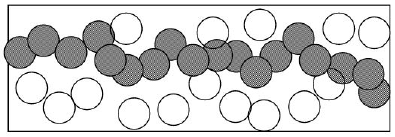
Energy-Efficient Approach:

Deploy redundant sensors (many more than needed), then use duty cycling.

Rotation Schedule:

To maximize lifetime, rotate active sensors:

Round 1: Sensors {1, 3, 5, 7} active (cover 100%)
Round 2: Sensors {2, 4, 6, 8} active (cover 100%)
Round 3: Back to {1, 3, 5, 7}
...

Lifetime Improvement: If 50% of sensors needed for coverage, lifetime doubles through rotation.

NoteKnowledge Check: Area Coverage Optimization

viewof kcWsnCov3 = {
  const container = html`<div id="kc-wsn-cov-3-container"></div>`;
  if (container && typeof InlineKnowledgeCheck !== 'undefined') {
    container.innerHTML = '';
    container.appendChild(InlineKnowledgeCheck.create({
      question: "An environmental monitoring WSN covers a 1km squared area with 400 temperature sensors (Rs = 25m). Analysis shows only 160 sensors are needed for complete coverage. The network lifetime with all 400 active is 6 months. What coverage rotation strategy maximizes network lifetime?",
      options: [
        {text: "Keep all 400 sensors active - more sensors means better data quality and no coverage gaps", correct: false, feedback: "Incorrect. Keeping redundant sensors active wastes energy with minimal coverage benefit. 400 sensors provide excessive overlap when only 160 are needed. While data redundancy can improve accuracy through averaging, the 2.5x energy waste (400 vs 160 active) drastically shortens lifetime to just 6 months. For long-term environmental monitoring, extended lifetime through rotation scheduling is far more valuable than marginal data quality improvements."},
        {text: "Two-round rotation: Round 1 activates 160 sensors, Round 2 activates different 160 sensors, alternating daily leads to 12-month lifetime", correct: false, feedback: "Incorrect. While rotation is the right approach, you haven't used all available sensors. With 400 total sensors and 160 needed per round, you can create 400/160 = 2.5 rounds, not just 2. By limiting to 2 rounds of 160 sensors each, you only utilize 320 sensors, leaving 80 unused. This achieves 2x lifetime improvement (12 months) but misses potential for further optimization."},
        {text: "Random activation: Each day, randomly select 160 sensors to activate - ensures fair energy distribution", correct: false, feedback: "Incorrect. Random activation has critical flaws: (1) No coverage guarantee - random selection might create coverage holes by chance, (2) Communication overhead - daily reconfiguration requires coordination messages, (3) No benefit over deterministic rotation - randomness doesn't improve lifetime if you're selecting the same count (160) daily. Deterministic rotation schedules provide predictable coverage with zero runtime overhead."},
        {text: "Optimal rotation: Create 2.5 rounds using 160 + 160 + 80 sensors leads to 15-month lifetime (2.5x improvement)", correct: true, feedback: "Correct! Optimal rotation strategy maximizes utilization of all 400 sensors: (1) Round 1: Activate 160 sensors for 6 months, (2) Round 2: Activate different 160 sensors for 6 months, (3) Round 3: Activate remaining 80 sensors + partial reuse of first 80 from Round 1 for 3 months. Total lifetime = 6 + 6 + 3 = 15 months vs. 6 months all-active (2.5x improvement). Implementation: During deployment, sensors are assigned to coverage sets using OGDC or similar algorithms. Each set provides complete coverage independently."}
      ],
      difficulty: "medium",
      topic: "area-coverage-rotation"
    }));
  }
  return container;
}

365.3.2 Point Coverage

Objective: Monitor a discrete set of critical points (not continuous area).

%% fig-alt: "Point coverage model showing discrete critical points monitored by sensors within sensing range, illustrating set cover problem"
%%{init: {'theme': 'base', 'themeVariables': {'primaryColor': '#2C3E50', 'primaryTextColor': '#fff', 'primaryBorderColor': '#16A085', 'lineColor': '#16A085', 'secondaryColor': '#E67E22', 'tertiaryColor': '#ECF0F1', 'fontSize': '16px'}}}%%
graph TD
    subgraph "Point Coverage Model"
        POINTS["Points of Interest<br/>P = {p1, p2, ..., pn}"]

        P1["Point p1<br/>(Door)"]
        P2["Point p2<br/>(Window)"]
        P3["Point p3<br/>(Valve)"]
        P4["Point p4<br/>(Junction)"]

        S1["Sensor s1<br/>Range Rs"]
        S2["Sensor s2<br/>Range Rs"]
        S3["Sensor s3<br/>Range Rs"]

        CHECK{"All points<br/>covered?"}

        SUCCESS["Point Coverage<br/>Achieved"]
        FAIL["Add sensors"]
    end

    POINTS --> P1
    POINTS --> P2
    POINTS --> P3
    POINTS --> P4

    S1 -.->|"d(p1,s1) <= Rs"| P1
    S1 -.->|"d(p2,s1) <= Rs"| P2
    S2 -.->|"d(p2,s2) <= Rs"| P2
    S2 -.->|"d(p3,s2) <= Rs"| P3
    S3 -.->|"d(p3,s3) <= Rs"| P3
    S3 -.->|"d(p4,s3) <= Rs"| P4

    P1 --> CHECK
    P2 --> CHECK
    P3 --> CHECK
    P4 --> CHECK

    CHECK -->|"Yes"| SUCCESS
    CHECK -->|"No"| FAIL

    SUCCESS -.-> KCOV["K-Coverage:<br/>Each point covered<br/>by >= k sensors"]

    style POINTS fill:#2C3E50,stroke:#16A085,stroke-width:3px,color:#fff
    style P1 fill:#E67E22,stroke:#2C3E50,stroke-width:2px,color:#fff
    style P2 fill:#E67E22,stroke:#2C3E50,stroke-width:2px,color:#fff
    style P3 fill:#E67E22,stroke:#2C3E50,stroke-width:2px,color:#fff
    style P4 fill:#E67E22,stroke:#2C3E50,stroke-width:2px,color:#fff
    style S1 fill:#16A085,stroke:#2C3E50,stroke-width:3px,color:#fff
    style S2 fill:#16A085,stroke:#2C3E50,stroke-width:3px,color:#fff
    style S3 fill:#16A085,stroke:#2C3E50,stroke-width:3px,color:#fff
    style CHECK fill:#3498DB,stroke:#2C3E50,stroke-width:3px,color:#fff
    style SUCCESS fill:#D5F4E6,stroke:#16A085,stroke-width:3px
    style FAIL fill:#FADBD8,stroke:#E74C3C,stroke-width:3px
    style KCOV fill:#ECF0F1,stroke:#2C3E50,stroke-width:2px

Figure 365.2: Point coverage model showing discrete critical points monitored by sensors within sensing range, illustrating set cover problem

Applications: - Building access monitoring (doors, windows) - Pipeline monitoring (junctions, valves) - Bridge structural health monitoring (stress points) - Smart grid (critical substations)

Mathematical Formulation:

Let P = {p1, p2, …, pn} be points to cover:

\[ \forall p_i \in P, \exists s_j \in \text{Active} : d(p_i, s_j) \leq R_s \]

Minimum Sensor Placement:

This is the classic set cover problem (NP-hard).

NoteKnowledge Check: Point Coverage Set Cover

viewof kcWsnCov11 = {
  const container = html`<div id="kc-wsn-cov-11-container"></div>`;
  if (container && typeof InlineKnowledgeCheck !== 'undefined') {
    container.innerHTML = '';
    container.appendChild(InlineKnowledgeCheck.create({
      question: "A water utility monitors 100 critical valve locations across a city using WSN with Rs = 50m. Valve locations are sparse (average 200m apart). Initial grid deployment uses 500 sensors for complete area coverage. How can you reduce sensor count while maintaining valve monitoring?",
      options: [
        {text: "Keep area coverage approach - complete coverage guarantees all valves are monitored", correct: false, feedback: "Incorrect. Area coverage wastes sensors covering empty regions between valves. With valves 200m apart (sparse) and Rs=50m, area coverage requires sensors every ~87m (triangular lattice spacing sqrt(3) x Rs) across entire city. Point coverage focuses sensors only near 100 valve locations, potentially reducing to 100-150 sensors (88% reduction)."},
        {text: "Switch to point coverage with greedy set cover algorithm - deploy sensors only to cover 100 valve locations, ~100-150 sensors needed", correct: true, feedback: "Correct! Point coverage with set cover optimization dramatically reduces sensor count: (1) Problem formulation: Given 100 valve locations (points) and Rs=50m, find minimum sensors covering all valves, (2) Greedy algorithm: Repeatedly select sensor location covering most uncovered valves until all covered, (3) Sensor reduction: 100 valves with Rs=50m leads to ~100-150 sensors vs 500 area coverage sensors = 70-80% reduction."},
        {text: "Use mobile sensors that patrol between valves - 10 mobile sensors can cover 100 valves over time", correct: false, feedback: "Incorrect. Mobile sensors have critical limitations for critical infrastructure: (1) Coverage latency: 10 mobiles covering 100 valves means each visits valve every 10 time periods. Valve failures go undetected for 90% of time (unacceptable for critical monitoring), (2) Movement energy: Mobile platforms consume 10-100x more energy than static sensing."},
        {text: "Random deployment of 200 sensors - should cover most valves by chance", correct: false, feedback: "Incorrect. Random deployment for point coverage is inefficient and unreliable: (1) No coverage guarantee: Random scatter might leave 10-20 valves uncovered by chance (20% failure rate unacceptable for critical infrastructure), (2) Wasted sensors: Random placement clusters sensors in some areas while leaving gaps near critical valves."}
      ],
      difficulty: "medium",
      topic: "point-coverage-optimization"
    }));
  }
  return container;
}

365.3.3 K-Coverage and Redundancy

Critical applications require k-coverage: every point covered by at least k sensors (fault tolerance).

%% fig-alt: "K-coverage hierarchy showing 1-coverage (basic monitoring), 2-coverage (fault-tolerant with 1 failure tolerance), and 3-coverage (high reliability with 2 failure tolerance) with applications and cost trade-offs"
%%{init: {'theme': 'base', 'themeVariables': {'primaryColor': '#2C3E50', 'primaryTextColor': '#fff', 'primaryBorderColor': '#16A085', 'lineColor': '#16A085', 'secondaryColor': '#E67E22', 'tertiaryColor': '#ECF0F1', 'fontSize': '16px'}}}%%
graph TD
    subgraph "K-Coverage Hierarchy"
        KCOV["K-Coverage<br/>Redundancy"]

        K1["1-Coverage<br/>(Basic)"]
        K2["2-Coverage<br/>(Redundant)"]
        K3["3-Coverage<br/>(High Reliability)"]

        K1_DESC["Each point monitored<br/>by >= 1 sensor"]
        K2_DESC["Each point monitored<br/>by >= 2 sensors<br/>(Tolerates 1 failure)"]
        K3_DESC["Each point monitored<br/>by >= 3 sensors<br/>(Tolerates 2 failures)"]

        K1_APP["Applications:<br/>Environmental monitoring<br/>Non-critical sensing"]
        K2_APP["Applications:<br/>Industrial monitoring<br/>Smart buildings"]
        K3_APP["Applications:<br/>Critical infrastructure<br/>Security systems"]
    end

    KCOV --> K1
    KCOV --> K2
    KCOV --> K3

    K1 --> K1_DESC
    K2 --> K2_DESC
    K3 --> K3_DESC

    K1_DESC -.-> K1_APP
    K2_DESC -.-> K2_APP
    K3_DESC -.-> K3_APP

    K1_APP -.->|"Cost: N sensors"| COST1["Lowest cost"]
    K2_APP -.->|"Cost: 2N sensors"| COST2["Medium cost<br/>2x reliability"]
    K3_APP -.->|"Cost: 3N sensors"| COST3["High cost<br/>3x reliability"]

    style KCOV fill:#2C3E50,stroke:#16A085,stroke-width:3px,color:#fff
    style K1 fill:#16A085,stroke:#2C3E50,stroke-width:3px,color:#fff
    style K2 fill:#E67E22,stroke:#2C3E50,stroke-width:3px,color:#fff
    style K3 fill:#E74C3C,stroke:#2C3E50,stroke-width:3px,color:#fff
    style K1_DESC fill:#D5F4E6,stroke:#2C3E50,stroke-width:2px
    style K2_DESC fill:#FADBD8,stroke:#2C3E50,stroke-width:2px
    style K3_DESC fill:#F5B7B1,stroke:#2C3E50,stroke-width:2px
    style K1_APP fill:#ECF0F1,stroke:#2C3E50,stroke-width:1px
    style K2_APP fill:#ECF0F1,stroke:#2C3E50,stroke-width:1px
    style K3_APP fill:#ECF0F1,stroke:#2C3E50,stroke-width:1px
    style COST1 fill:#D5F4E6,stroke:#16A085,stroke-width:2px
    style COST2 fill:#FADBD8,stroke:#E67E22,stroke-width:2px
    style COST3 fill:#F5B7B1,stroke:#E74C3C,stroke-width:2px

Figure 365.3: K-coverage hierarchy showing 1-coverage, 2-coverage, and 3-coverage levels with applications and cost trade-offs

K-Coverage Levels:

1-coverage: Each point monitored by >= 1 sensor
2-coverage: Each point monitored by >= 2 sensors (tolerates 1 failure)
k-coverage: Each point monitored by >= k sensors (tolerates k-1 failures)

NoteKnowledge Check: K-Coverage and Redundancy

viewof kcWsnCov4 = {
  const container = html`<div id="kc-wsn-cov-4-container"></div>`;
  if (container && typeof InlineKnowledgeCheck !== 'undefined') {
    container.innerHTML = '';
    container.appendChild(InlineKnowledgeCheck.create({
      question: "A chemical plant monitors 20 critical pressure points with WSN sensors (Rs = 15m). Regulations require the system to tolerate 2 simultaneous sensor failures without losing monitoring of any critical point. What is the minimum k-coverage level required, and approximately how many sensors are needed?",
      options: [
        {text: "2-coverage with approximately 40 sensors - tolerates 2 failures since each point covered by 2 sensors", correct: false, feedback: "Incorrect. K-coverage tolerates (k-1) failures, not k failures. With 2-coverage, each point is monitored by at least 2 sensors, so if 1 sensor fails, 1 sensor remains (tolerates 1 failure). But if 2 sensors covering the same point fail simultaneously, that point becomes unmonitored. You need k >= 3 to tolerate 2 failures."},
        {text: "3-coverage with approximately 60 sensors - tolerates 2 failures since 3-coverage survives when up to 2 covering sensors fail", correct: true, feedback: "Correct! K-coverage provides (k-1) failure tolerance, so 3-coverage tolerates 2 failures: (1) Each critical point is covered by at least 3 sensors, (2) If 2 sensors fail, at least 1 sensor remains operational covering that point, (3) Sensor count calculation: 20 points x 3 sensors per point = 60 sensors (approximate, assuming minimal overlap)."},
        {text: "1-coverage with 20 sensors plus automatic reconfiguration - if sensors fail, nearby sensors adjust sensing range", correct: false, feedback: "Incorrect. Sensors have fixed sensing range (Rs) determined by hardware physics - they cannot adjust sensing range dynamically. Additionally, 1-coverage with 20 sensors provides zero fault tolerance - any single sensor failure creates an unmonitored point."},
        {text: "4-coverage with approximately 80 sensors - higher k is safer for critical chemical monitoring", correct: false, feedback: "Incorrect. While 4-coverage would indeed provide higher reliability (tolerates 3 failures), it exceeds the stated requirement of tolerating 2 failures. This results in 33% cost increase (80 vs 60 sensors) with no additional value toward meeting the specification."}
      ],
      difficulty: "medium",
      topic: "k-coverage-redundancy"
    }));
  }
  return container;
}

365.3.4 Barrier Coverage

Figure 365.4: Barrier Coverage concept - sensors deployed to detect intruders crossing a border or perimeter, ensuring no gaps in detection line

Objective: Detect intruders crossing a barrier (line or belt).

%% fig-alt: "Barrier coverage model showing sensors deployed along border to detect intruder crossings with overlapping sensing zones"
%%{init: {'theme': 'base', 'themeVariables': {'primaryColor': '#2C3E50', 'primaryTextColor': '#fff', 'primaryBorderColor': '#16A085', 'lineColor': '#16A085', 'secondaryColor': '#E67E22', 'tertiaryColor': '#ECF0F1', 'fontSize': '16px'}}}%%
graph LR
    subgraph "Barrier Coverage Model"
        BORDER_START["Border<br/>Start"]

        S1["Sensor 1<br/>Range Rs"]
        S2["Sensor 2<br/>Range Rs"]
        S3["Sensor 3<br/>Range Rs"]
        S4["Sensor 4<br/>Range Rs"]

        BORDER_END["Border<br/>End"]

        INTRUDER["Intruder Path<br/>(Any crossing)"]
    end

    BORDER_START --> S1
    S1 --> S2
    S2 --> S3
    S3 --> S4
    S4 --> BORDER_END

    INTRUDER -.->|"Must cross >= k<br/>sensor ranges"| S2
    INTRUDER -.->|"Detection"| S3

    S1 -.->|"Sensing coverage"| COV1["Coverage<br/>zone"]
    S2 -.->|"Sensing coverage"| COV2["Coverage<br/>zone"]
    S3 -.->|"Sensing coverage"| COV3["Coverage<br/>zone"]
    S4 -.->|"Sensing coverage"| COV4["Coverage<br/>zone"]

    style BORDER_START fill:#2C3E50,stroke:#16A085,stroke-width:3px,color:#fff
    style BORDER_END fill:#2C3E50,stroke:#16A085,stroke-width:3px,color:#fff
    style S1 fill:#16A085,stroke:#2C3E50,stroke-width:3px,color:#fff
    style S2 fill:#16A085,stroke:#2C3E50,stroke-width:3px,color:#fff
    style S3 fill:#16A085,stroke:#2C3E50,stroke-width:3px,color:#fff
    style S4 fill:#16A085,stroke:#2C3E50,stroke-width:3px,color:#fff
    style INTRUDER fill:#E74C3C,stroke:#2C3E50,stroke-width:3px,color:#fff
    style COV1 fill:#D5F4E6,stroke:#2C3E50,stroke-width:1px
    style COV2 fill:#D5F4E6,stroke:#2C3E50,stroke-width:1px
    style COV3 fill:#D5F4E6,stroke:#2C3E50,stroke-width:1px
    style COV4 fill:#D5F4E6,stroke:#2C3E50,stroke-width:1px

Figure 365.5: Barrier coverage model showing sensors deployed along border to detect intruder crossings with overlapping sensing zones

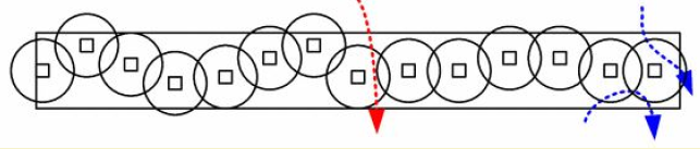
Applications: - Border surveillance - Perimeter security (military bases, critical infrastructure) - Wildlife corridor monitoring - Pipeline intrusion detection

365.3.5 K-Barrier Coverage Levels

%% fig-alt: "K-barrier coverage hierarchy showing 1-barrier, 2-barrier, and k-barrier levels with weak and strong variants and their applications"
%%{init: {'theme': 'base', 'themeVariables': {'primaryColor': '#2C3E50', 'primaryTextColor': '#fff', 'primaryBorderColor': '#16A085', 'lineColor': '#16A085', 'secondaryColor': '#E67E22', 'tertiaryColor': '#ECF0F1', 'fontSize': '16px'}}}%%
graph TD
    subgraph "K-Barrier Coverage Hierarchy"
        ROOT["Barrier<br/>Coverage"]

        LEVEL1["1-Barrier<br/>Coverage"]
        LEVEL2["2-Barrier<br/>Coverage"]
        LEVELK["K-Barrier<br/>Coverage"]

        WEAK["Weak k-Barrier:<br/>Path intersects<br/>>= k sensor ranges"]
        STRONG["Strong k-Barrier:<br/>Every point on path<br/>covered by >= k sensors"]

        APP1["Basic detection<br/>Perimeter monitoring"]
        APP2["Redundant detection<br/>Critical infrastructure"]
        APPK["High security<br/>Military borders"]
    end

    ROOT --> LEVEL1
    ROOT --> LEVEL2
    ROOT --> LEVELK

    LEVEL1 --> APP1
    LEVEL2 --> APP2
    LEVELK --> APPK

    LEVEL2 -.-> WEAK
    LEVEL2 -.-> STRONG

    WEAK -.->|"Fewer sensors<br/>Lower cost"| WEAK_TRADE["Detection at<br/>k points"]
    STRONG -.->|"More sensors<br/>Higher cost"| STRONG_TRADE["Continuous<br/>tracking"]

    style ROOT fill:#2C3E50,stroke:#16A085,stroke-width:3px,color:#fff
    style LEVEL1 fill:#16A085,stroke:#2C3E50,stroke-width:3px,color:#fff
    style LEVEL2 fill:#E67E22,stroke:#2C3E50,stroke-width:3px,color:#fff
    style LEVELK fill:#E74C3C,stroke:#2C3E50,stroke-width:3px,color:#fff
    style WEAK fill:#AED6F1,stroke:#2C3E50,stroke-width:2px
    style STRONG fill:#F9E79F,stroke:#2C3E50,stroke-width:2px
    style APP1 fill:#D5F4E6,stroke:#2C3E50,stroke-width:2px
    style APP2 fill:#FADBD8,stroke:#2C3E50,stroke-width:2px
    style APPK fill:#F5B7B1,stroke:#2C3E50,stroke-width:2px
    style WEAK_TRADE fill:#ECF0F1,stroke:#2C3E50,stroke-width:1px
    style STRONG_TRADE fill:#ECF0F1,stroke:#2C3E50,stroke-width:1px

Figure 365.6: K-barrier coverage hierarchy showing 1-barrier, 2-barrier, and k-barrier levels with weak and strong variants

365.3.6 Weak vs. Strong Barrier

Weak k-Barrier:

Figure 365.7: Weak k-Barrier Coverage - Crossing paths intersect at least k sensor ranges, though gaps may exist along the path

Every path crossing the barrier intersects sensing ranges of at least k sensors.

Strong k-Barrier:

Figure 365.8: Strong k-Barrier Coverage - Every point along crossing paths is covered by at least k sensors simultaneously, providing robust intruder detection

Every point on every path crossing the barrier is within sensing range of at least k sensors simultaneously.

Deployment Strategy:

For a barrier of length L with sensors of range Rs:

Minimum sensors for 1-barrier: ceil(L / (2 x Rs))

Minimum sensors for k-barrier: Approximately k x ceil(L / (2 x Rs))

NoteKnowledge Check: Barrier Coverage Design

viewof kcWsnCov5 = {
  const container = html`<div id="kc-wsn-cov-5-container"></div>`;
  if (container && typeof InlineKnowledgeCheck !== 'undefined') {
    container.innerHTML = '';
    container.appendChild(InlineKnowledgeCheck.create({
      question: "A national park needs to monitor a 1.2km wildlife migration corridor to count animals passing through. Sensors have Rs = 20m. The requirement is to detect that animals crossed (presence detection), but continuous position tracking is not needed. Budget is limited. What barrier coverage should you deploy?",
      options: [
        {text: "Strong 2-barrier coverage with approximately 120 sensors - ensures complete continuous monitoring with redundancy", correct: false, feedback: "Incorrect. Strong 2-barrier provides continuous tracking capability (every point along every crossing path covered by 2+ sensors simultaneously), which exceeds requirements. The scenario only needs presence detection (did animal cross?), not position tracking (where is animal right now?). Strong 2-barrier requires ~120 sensors (2 layers x 60 sensors/layer), while weak 1-barrier needs only ~30 sensors - 4x cost difference."},
        {text: "Weak 1-barrier coverage with approximately 30 sensors - minimal cost while guaranteeing every crossing path intersects at least one sensor", correct: true, feedback: "Correct! Weak 1-barrier is optimal for this requirement: (1) Detection guarantee: Every crossing path must intersect at least 1 sensor's range, ensuring animals are detected, (2) Sensor count: L/(2 x Rs) = 1200m/(2 x 20m) = 30 sensors, (3) Cost optimization: Minimal sensor count meeting detection requirement."},
        {text: "Strong 1-barrier coverage with approximately 60 sensors - guarantees complete continuous coverage along entire corridor", correct: false, feedback: "Incorrect. While strong 1-barrier provides continuous coverage (every point on crossing paths monitored), it's costlier than weak 1-barrier (60 vs 30 sensors) without addressing the stated requirement. The scenario needs detection (count animals), not tracking (monitor position continuously)."},
        {text: "Area coverage of entire 1.2km corridor - only comprehensive monitoring guarantees detection of all crossing paths", correct: false, feedback: "Incorrect. Area coverage is massive overkill for linear barrier monitoring. To cover 1.2km x 40m corridor with Rs=20m requires ~150+ sensors vs. 30 sensors for weak barrier. Barrier coverage exploits the linear geometry - you only care about detecting crossings perpendicular to corridor axis."}
      ],
      difficulty: "medium",
      topic: "barrier-coverage-types"
    }));
  }
  return container;
}

365.4 Coverage Type Comparison

Coverage Type	Goal	Sensors Needed	Applications
Area	Monitor every point in 2D region	High (full coverage)	Environmental, agriculture
Point	Monitor discrete critical locations	Low (targeted)	Infrastructure, access control
Barrier	Detect border crossings	Medium (linear)	Security, wildlife
K-Coverage	Redundancy for fault tolerance	K x base sensors	Critical systems

365.5 Summary

This chapter covered the three main types of WSN coverage problems:

Key Takeaways:

1. Area Coverage - Monitor continuous 2D regions using rotation scheduling to maximize lifetime. Best for environmental monitoring where events can occur anywhere.

2. Point Coverage - Monitor discrete critical locations using set cover algorithms. Dramatically reduces sensor count compared to area coverage for sparse infrastructure.

3. Barrier Coverage - Detect crossings using weak (path-intersection) or strong (continuous monitoring) strategies. Choose based on detection vs tracking requirements.

4. K-Coverage - Provides (k-1) failure tolerance. Match k to reliability requirements: k=1 for basic, k=2 for fault tolerance, k=3+ for critical systems.

365.6 What’s Next?

Now that you understand coverage types, the next chapter explores algorithms for maintaining coverage efficiently.

Continue to WSN Coverage Algorithms - Learn about crossing theory, OGDC, and virtual force algorithms for coverage optimization.